3 The FMAPE algorithm with variable
hyperparameter

3.1 The Bayesian approach

  We use the Bayesian strategy to obtain an iterative algorithm for image reconstruction. The application of Bayes' theorem to the image reconstruction problem gives:

 

$${\bf P}({\bf a}\vert{\bf p}) = \frac{{\bf P}({\bf p}\vert{\bf a}){\bf P}({\bf a})}{{\bf P}({\bf p})}\;\;.$$ (2)

The most probable image ${\bf a}$, given data ${\bf p}$, is obtained by maximizing ${\bf P}({\bf a}\vert{\bf p})$ in (2) or the product ${\bf P}({\bf p}\vert{\bf a}){\bf P}({\bf a})$ since ${\bf P}({\bf p})$ is constant.

3.2 The likelihood

The conditional probability ${\bf P}({\bf p}\vert{\bf a})$ describes the noise in the data and its possible object dependence. It is fully specified in the problem by the likelihood function. As indicated above, we have two independent processes: image formation on the detector array and detector readout. Taking the two processes into account, the compound likelihood is (Núñez & Llacer 1993a):

$${\bf L} = {\bf P}({\bf p}\vert{\bf a}) = \prod_{j=1}^{D} \su... ...c{(k-p_j)^2}{2\sigma^2}} {\rm e}^{-h_j}\;\;\frac{(h_j)^{k}}{k!}$$

and its logarithm is:

$$\begin{eqnarray} \log {\bf L} & = & \sum_{j=1}^{D}{\left[-\log(\sqrt{2\pi}\sigma... ...ac{(k-p_j)^2}{2\sigma^2}}\; \frac{(h_j)^k}{k!}\right)}\right]\;\;.\end{eqnarray}$$ (3)

This compound likelihood was first introduced for reconstructions of Poisson data in the presence of readout noise by Llacer & Núñez (1990). Snyder et al. (1993a) use the same likelihood form for CCD cameras. If the process were pure Poisson (no readout noise), the logarithm of the likelihood would be the classical expression:

 

$$\log {\bf L} = \sum_{j=1}^{D}{\left[- h_j +p_j\log h_j -\log (p_j!)\right]}\;\;.$$ (4)

3.3 The prior

We use entropy to define the prior probability ${\bf P}({\bf a})$ in a generalization of the concepts originally described by Frieden (1972).

Let N be the total energy (usually the number of counts or photons) in the object. Assume that there is an intensity increment $\Delta a$describing an intensity jump to which we can assign some appropriate physical meaning. Frieden (1972) describes $\Delta a$ as the finest known intensity jumps that are possible in the object, but we prefer to relax that definition and consider it an adjustable hyperparameter of the Bayesian function.

Assume, in addition, that we have prior information regarding the statistical makeup of the object obtained, for example, from previous observations or from observations at other wavelengths from which one could infere realistic information about the makeup of the object at the wavelength at which the observation is made. If $Q_i\;\;i=1,\cdots,B$ is the prior energy distribution, the prior probability of a photon going to pixel i is given by:

$$g_i = \frac{Q_i}{\sum_{l=1}^{B} Q_l}\;\;.$$

In that case, the a priori source probability of $\frac{N}{\Delta a}$quanta distributing randomly over the B pixels is then characterized by the multinomial law (Lloyd 1980; Handbook of Applicable Mathematics, Vol II, p. 92) as:  

$$P({\bf a}) = \frac{(N/\Delta a)!}{\prod_{i=1}^{B}(a_i/\Delta a)!}\prod_{i=1}^{B}(g_i)^{a_i/\Delta a}\;\;.$$ (5)

The a priori probability $P({\bf a})$ of (5) reflects the statistical distribution process of source units $\frac{a_i}{\Delta a}$given the a priori probabilistic information map g_i.

If the prior information is not reliable, it is best to ignore it and give a uniform value to $Q_i = \frac{\sum_{l=1}^{B} Q_l}{B}$ that means g_i = 1/B. In that case, the multinomial distribution of (5) reduces to a normalized version of the Boltzmann distribution used by Frieden (1972).

Assume, also, that the intensity increment $\Delta a$ is space variant in the object space. The introduction of the variability of $\Delta a$ is the core of this paper. The parameter $\Delta a$ controls the amount of prior information that is introduced into the solution. If the values of Q_i represent a uniform field, the parameter $\Delta a$ will control the degree of smoothness of the solution. Its spatial variability will allow the local control of smoothness avoiding noise amplification in the different areas of the image.

Let $\Delta a_i\;\; i=1,\cdots,B$ be the variable increment. Now, in place of $\frac{N}{\Delta a}$ units we distribute $\sum_{i=1}^{B} {\frac{a_i}{\Delta a_i}}$ units. The a priori source probability of $\sum_{i=1}^{B} {\frac{a_i}{\Delta a_i}}$ quanta distributing randomly over the B pixels is then:

 

$$P({\bf a}) =\frac{( \sum_{i=1}^{B}{\frac {a_i}{\Delta a_i}})... ...{a_i}{\Delta a_i})!} \prod_{i=1}^{B}(g_i)^{a_i/\Delta a_i}\;\;.$$ (6)

A natural choice for the prior energy distribution is:  

$$g_i = \frac{\frac{Q_i}{\Delta a_i}}{\sum_{i=1}^{B} \frac{Q_i}{\Delta a_i}}\;\;.$$ (7)

Taking logarithms in (6)

$$\begin{eqnarray} \log {\bf P}({\bf a}) & = & \log \biggl( \sum_{i=1}^{B}{\frac {... ...iggr)! +\\ & & + \sum_{i=1}^{B} \frac{a_i}{\Delta a_i} \log g_i\;.\end{eqnarray}$$

To compute the factorials, we use Stirling's approximation

 

$$x! = (2\pi x)^{1\over 2} x^x {\rm e}^{-x};\;\;\; \log(x!) \approx x \log x - x$$ (8)

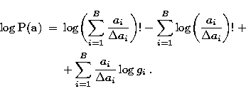
in which we discarded the term ${1\over 2} \log 2\pi x$. This approximation is adequate for x > 10. Also, the use of the complete approximation would give a term in ${1\over x}$ in the algorithms that would produce a numerical instability at the background pixels. In some cases (p.e. in regions of very low flux or background in photon counting devices) the approximation used may produce some error but we prefer to use this approximation to avoid the menctioned numerical instability. Using (10)

$$\begin{eqnarray} \log {\bf P}({\bf a}) & = & \biggl( \sum_{i=1}^{B}{\frac {a_i}{... ...right]} + \\ & & + \sum_{i=1}^{B} \frac {a_i}{\Delta a_i} \log g_i\end{eqnarray}$$

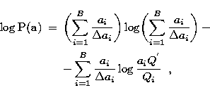
and taking into account (7) the logarithm of the probability ${\bf P}({\bf a})$ is:

$$\begin{eqnarray} \log {\bf P}({\bf a}) & = & \biggl( \sum_{i=1}^{B}{\frac {a_i}{... ...um_{i=1}^{B}{\frac{a_i}{\Delta a_i}\log\frac{a_i Q^{'}}{Q_i}}\;\;,\end{eqnarray}$$ (9)

where

$$Q^{'} = \sum_{i=1}^{B} \frac{Q_i}{\Delta a_i}\;\;.$$

If we do not consider the space variation of the intensity increment i.e. $\Delta a = {\rm const.}$, and taking into account that both $\sum{a_i}$ and $\sum{Q_i}$ are constant, the log of the prior probability is:  

$$\log {\bf P}({\bf a}) = - \sum_{i=1}^{B}{\frac{a_i}{\Delta a}\log\frac{a_i}{Q_i}} + {\rm const.}\;\;{\rm terms.}$$ (10)

This form of the entropy that includes the parameter $\Delta a$ and the spatial prior information ${\bf Q}$ is often called cross-entropy.

3.4 The general algorithm

As discussed in Sect. 3.1, the maximum a posteriori (MAP) probability will be obtained by maximizing ${\bf P}({\bf a}\vert{\bf p}) = {\bf P}({\bf a}){\bf P}({\bf p}\vert{\bf a})$, or equivalently, the logarithm of that probability, $\log {\bf P}({\bf a}\vert{\bf p}) = \log {\bf P}({\bf a}) + \log {\bf L}$ with the constraint of energy conservation:

 

$$\sum_{i=1}^{B}{q_i a_i} = \sum_{j=1}^{D}{p_j} - \sum_{j=1}^{D}{b_j}\;\;.$$ (11)

Taking into account (3), (14) and (16), the Bayesian function to be maximized is:

$$BY = ( \sum_{i=1}^{B}{\frac {a_i}{\Delta a_i}}) \log ( \sum_... ..._{i=1}^{B}{\frac{a_i}{\Delta a_i}\log\frac{a_i Q^{'}}{Q_i}}\; +$$

$$+\sum_{j=1}^{D}{\left[-\log(\sqrt{2\pi}\sigma) - h_j + \log\... ...{(k-p_j)^2}{2\sigma^2}}\; \frac{(h_j)^k}{k!}\right)}\right]} -$$

 

$$- \mu \left(\sum_{i=1}^{B}{q_i a_i} - \sum_{j=1}^{D}{p_j} + \sum_{j=1}^{D}{b_j}\right)\;\;,$$ (12)

where h_j is given by:

$$h_j = \sum_{i=1}^{B}{f^{'}_{ji}a_i} + b_j$$

and $\mu$ is a Lagrange multiplier for the conserconservation of counts. Note that the relative weight of the two terms in the Bayesian function (17) is controlled by the set of hyperparameters $\Delta a_i$.

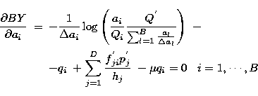
The nonlinear nature of the reconstruction problem described by (17) suggests an iterative algorithm. We have found that gradient methods, like steepest ascent or conjugate gradient algorithms, although well established, produce negative results for most of the pixels in the low light level part of the image. Also, the well-behaved Expectation Maximization (EM) algorithm -developed by Dempster et al. (1977) and extensively used for maximum likelihood reconstruction, after the work of Shepp & Vardi (1982)- is difficult to use in the Bayesian case with entropy because it requires the solution of transcendental equations in the M-step. Instead, we have found that the method of Successive Substitutions described by Hildebrand (1974) and Meinel (1986), and used by the authors in several previous papers, affords us greater flexibility than other methods and results in rapidly converging algorithms.

The Successive Substitutions method can be described as follows: given a series of equations on the unknowns $a_i,\cdots,a_B$ in the form

 

$$a_i = K F(\{a_m\}), \;\;\; i=1,\cdots,B$$ (13)

where F is some function, $(\{a_m\})$ is the complete set of variables $a_i,\cdots,a_B$, and K is a normalization constant, (18) can be transformed into a recursive relation by

 

$$a^{(k+1)}_i = K F(\{a^{(k)}_m\}), \;\;\; i=1,\cdots, B\;\;.$$ (14)

Each of the new values of a^(k+1)_i is calculated from all the known B values of $\{a^{(k)}_m\}$, and the complete set is updated at once. The constant K is obtained by invoking the energy conservation law:

 

$$\sum_{i=1}^{B}{q_i a^{(k+1)}_i} = \sum_{i=1}^{B}{Kq_iF(\{a^{(k)}_i\})} = \sum_{j=1}^{D}{p_j} - \sum_{j=1}^{D}{b_j}\;\;.$$ (15)

To obtain the maximum of (17), we set $\partial BY/\partial a_i = 0$, taking into account that

$$\frac{\partial l}{\partial a_i} = \frac{\partial l}{\partial... ...rtial a_i} = \frac{\partial l}{\partial h_j} f^{'}_{ji} \;\;\;,$$

$$\begin{eqnarray} \frac{\partial BY}{\partial a_i} & = & -\frac{1}{\Delta a_i} \l... ...\frac{k(h_j)^{k-1}}{k!}f^{'}_{ji} \right)} \right] -\mu q_i = 0\;.\end{eqnarray}$$

Multiplying and dividing by h_j in the last summation:

$$\begin{eqnarray} \frac{\partial BY}{\partial a_i} & = & -\frac{1}{\Delta a_i} \l... ...{\frac{f^{'}_{ji}p^{'}_j}{h_j}}\; -\mu q_i = 0 \;\;\; i=1,\cdots,B\end{eqnarray}$$ (16)

where

 

$$p^{'}_j = \frac{\sum_{k=0}^{\infty}{\left(\;k\; {\rm e}^{-\f... ...frac{(k-p_j)^2}{2\sigma^2}}\; \frac{(h_j)^k}{k!}\right)} }\;\;.$$ (17)

We could now solve for a_i in the first term of (22) and obtain a relation of the type of (18), but an exponential function would then appear. That exponential function causes instability in the solution (see, e.g., Núñez & Llacer 1990). Instead we divide Eq. (22) by q_i to obtain

$$-\frac{1}{q_i \Delta a_i} \log \left( \frac{a_i}{Q_i} \frac{Q^{'}}{\sum_{l=1}^{B}{\frac {a_l}{\Delta a_l}}}\right) +$$

$$+ \frac{1}{q_i}\sum_{j=1}^{D}{\frac{f^{'}_{ji}p^{'}_j}{\sum_... ...B}{f^{'}_{jl}a_l} + b_j}}\; = \mu + 1 \;\;\; i=1,\cdots,B \;\;.$$ (18)

Multiplying and dividing by C_j in the first summation, then adding a constant C to both sides of the equation, raising both sides to the power n, and finally multiplying both sides by a_i results in

$$\begin{eqnarray} a_i\left[\mu+1+C\right]^{n} & = & a_i\left[ \frac{1}{q_i}\sum_{... ...\Delta a_l}}}\right) + C\right]^{n} \nonumber \\ & & i=1,\cdots,B.\end{eqnarray}$$ (19)

The expression  (25) is of the type indicated by  (18). We can solve for the unknowns by the recursive relation (19), yielding the Bayesian maximum a posteriori algorithm with entropy prior (FMAPE) which is given by the iterative formula:

$$\begin{eqnarray} a^{(k+1)}_i & = & K a^{(k)}_i\left[ \frac{1}{q_i}\sum_{j=1}^{D}... ...lta a_l}}} \right) + C\right]^{n} \nonumber \\ & & i=1,\cdots,B.\end{eqnarray}$$ (20)

In the case of $\Delta a = {\rm const.}$, to compute $\log {\bf P}({\bf a})$in the Bayesian expresion (17) we should use (15) in place of (14). In that case, following the same steps as before, the algorithm (26) becomes:

$$\begin{eqnarray} a^{(k+1)}_i & = & K a^{(k)}_i\left[ \frac{1}{q_i}\sum_{j=1}^{D}... ...log \frac{a^{(k)}_i}{Q_i} + 1 \right) + C\right]^{n} i=1,\cdots B.\end{eqnarray}$$ (21)

In (26) and (27) k is the index of the iteration and K is a constant to conserve the energy by the relation $\sum_{i=1}^{B}q_ia_i = \sum_{j=1}^{D}p_j$, computed at the end of each iteration. Since

$$K = \frac{1}{\left[\mu+1+C\right]^{n}} \;\;\;,$$

computing the constant K is equivalent to computing the Lagrange multiplier $\mu$.

The iterative process defined by (26), (23) is the main result of this paper. We call this algorithm FMAPE. The algorithm has a number of desirable characteristics: It solves the cases of both pure Poisson data and Poisson data with Gaussian readout noise. The algorithm allows us to adjust the hyperparameters $\Delta a_i$ in order to determine the degree of smoothing in different regions or, in connection with known default images, to adjust the proximity between the reconstruction and the default image ${\bf Q}$. The algorithm maintains the positivity of the solution; it includes flatfield corrections; it removes background and can be accelerated to be faster than the Richardson-Lucy algorithm (Lucy 1974). The main loop (projection and backprojection) of the algorithm is similar in nature to the Expectation Maximization algorithm. The algorithm can be applied to a large number of imaging situations, including CCD and Pulse-counting cameras both in the presence and in the absence of background.

3.5 Positivity and Speed of convergence

The algorithm contains two arbitrary constants n and C. Both have been introduced in a way that the effect of changing the values of the constants n and C only affects the calculated values of K at the end of each iteration. The point of convergence of the algorithm (26), (23) is then solely dependent on the hyperparameters $\Delta a_i$. This can be seen as follows: Eq. (25) represents a set of B simultaneous equations in the unknowns a_i. Once the problem is solved by some appropriate method, Eq. (25) will hold, independently of the values of C and n. Equation (26) provides a method of solving the set of Eq. (25). If it converges to a solution of (25), that solution will therefore be independent of the values of C and n.

The constant C is introduced to insure the positivity of the solution. The presence of the negative entropy term

$$-\frac{1}{q_i \Delta a_i} \log \left( \frac{a^{(k)}_i Q^{'}}{Q_i \sum_{l=1}^{B}{\frac {a^{(k)}_l}{\Delta a_l}}} \right)$$

on the right hand of (26) means that the positivity of the solution is not automatically guaranteed unless an appropriate constant is introduced. As indicated above, different choices of C will not affect the convergence point. Such a problem is often present in maximum entropy approaches, either by gradient or EM algorithms.

Since the first term in (26) is always positive, a value of C somewhat larger than

$$\max \left[ -\frac{1}{q_i \Delta a_i} \log \left( \frac{a^{(... ...ac {a^{(k)}_l}{\Delta a_l}}} \right) \right] \;\;\;i=1,\cdots,B$$

will suffice. In practice, we find that changing C can affect the speed of convergence. Increasing C by a factor of 2 over the approximate smallest value necessary to maintain non-negativity results in slowing down convergence by approximately the same factor. The use of C=1 has usually resulted in adequate convergence speed and non-negativity of the pixels.

The constant n affects the rate of convergence. Since n affects the correction factor in (26), one can expect a range of values of n over which the iterative process is stable. We have observed that for n=1, the convergence rate improves by a factor of approximately n with respect to the rate for n=1. At the beginning of the process, when the correcting factors are rather high, a large n could result in an instability of the algorithm. After several iterations, when the correcting factors are close to unity, large values of n can be used. We have obtained stability using up to $n\approx 3$ at the beginning of the iterative process and larger values later.

3.6 The modified data p^'_j

  The complete form of the algorithm includes the computation of $p^{'}_j\;\;j=1,\cdots,D$ using (23) at each iteration. These variables were introduced in Llacer & Núñez (1990) for reconstructions in the presence of readout noise and further studied by Snyder et al. (1993a,b) and Núñez & Llacer (1993a). After every iteration, we must compute the modified data $p^{'}_j\;\;j=1,\cdots,D$ needed for the following iteration. This represents a pixel by pixel filtering operation in which the original data are substituted by a modified version.

In the absence of readout noise or when it is negligible, $\sigma \rightarrow 0$ in  (23). Then the exponentials are dominant at k=p_j and $p^{'}_j \rightarrow p_j$. We note that by its definition, $p^{'}_j\;\;j=1,\cdots,D$ is always positive, while the original data $p_j\;\;j=1,\cdots,D$ can be negative. For example, if the background is small, as in the case of the Hubble Space Telescope, the mean background is just above zero, but due to the readout noise, we may find a large number of pixels with negative values. Negative values are not allowed in any algorithm with projection-backprojection operations, like in the classical Richardson-Lucy algorithm. A preprocessing of the data or other approximations are common. We do not need any approximation or preprocessing. In fact, $p^{'}_j\;\;j=1,\cdots,D$ is a representation of the data that is positive and close to the data, with a degree of closeness that depends on the projections $h_j\;\;j=1,\cdots,D$ and $\sigma$. In this sense $p^{'}_j\;\;j=1,\cdots,D$ can be considered as a Bayesian filtered version of the data.

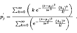
The practical computation of $p^{'}_j\;\;j=1,\cdots,D$ by Eq. (23) is not a trivial problem of numerical analysis. The p^'_js are numbers in the same range of the data, but to compute them, we need to compute summations from to $\infty$. In addition, exponentials and factorials can easily give either machine overflow or underflow, even using quadruple precision. To solve the problem Snyder et al. (1993b) use Poisson and saddlepoint approximations. We preferred to use a recursive technique without any approximation with very good results. Also, it is easy to see that the summations from k=0 to $\infty$ can be reduced to summations from $k=\max(0,p_j-n\sigma)$ to $k=p_j+n\sigma$ with $n\approx 3$ without loss of precision. By using this method, we can compute the p^'_j values with high accuracy, without increasing the CPU time apreciably.

3.7 Maximum likelihood algorithms

We can obtain a maximum likelihood algorithm from the general FMAPE by taking the limit when $\Delta~a_i~\rightarrow~\infty \;\; i=1,\cdots,B$.In that case the weight of the prior information (cross-entropy term) in the Bayesian function (17) is zero and the solution becomes a Maximum Likelihood one. The algorithm for the maximum likelihood (MLE) case in the presence of readout noise and background is:

$$\begin{eqnarray} a^{(k+1)}_i & = & K a^{(k)}_i\left[ \frac{1}{q_i}\sum_{j=1}^{D}... ...}a^{(k)}_l} + C_jb_j}}\;\right]^{n} \nonumber \\ & & i=1,\cdots,B,\end{eqnarray}$$ (22)

where p^'_j is given by Eq. (23).

In the case of no background and no readout noise, algorithm (28) becomes:

 

$$a^{(k+1)}_i = a^{(k)}_i\left[ \frac{1}{q_i}\sum_{j=1}^{D}{\f... ...\sum_{l=1}^{B}{f_{jl}a^{(k)}_l} }}\;\right]^{n}\; i=1,\cdots,B.$$ (23)

For n=1 and disregarding the gain (flatfield) corrections (q_i=1), (29) is identical to the Richardson-Lucy algorithm.