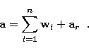
The hyperparameters ![]() have a fundamental role in the
Bayesian framework. They determine the relative weight between the prior
information and the likelihood in the Bayesian function and therefore
determine the chosen solution between the default image and the maximum
likelihood solution. Ultimately, they define the degree of smoothness of
the solution.
have a fundamental role in the
Bayesian framework. They determine the relative weight between the prior
information and the likelihood in the Bayesian function and therefore
determine the chosen solution between the default image and the maximum
likelihood solution. Ultimately, they define the degree of smoothness of
the solution.
If we use a single value for all the hyperparameters (![]() ), we could obtain a reasonable global fit of the
data, but the parts of the reconstructed image with low light levels
would appear noisy (over-reconstructed) while bright objects (stars)
would be too smooth (under-reconstructed). This effect is also present
in the Richardson-Lucy algorithm when stopped according to some
appropriate stopping rule and can easily be observed in the
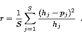
normalized residuals comparing the projection of the solution and the
data. To compute the normalized residual over a set of S detectors we
use the expression:
), we could obtain a reasonable global fit of the
data, but the parts of the reconstructed image with low light levels
would appear noisy (over-reconstructed) while bright objects (stars)
would be too smooth (under-reconstructed). This effect is also present
in the Richardson-Lucy algorithm when stopped according to some
appropriate stopping rule and can easily be observed in the
normalized residuals comparing the projection of the solution and the
data. To compute the normalized residual over a set of S detectors we
use the expression:
 |
(24) |
The FMAPE algorithm avoids noise amplification by the use of a
set of space-variant hyperparameters. A variable ![]() allows different degrees of smoothing in different regions,
ranging from very smooth (or very similar to the prior
allows different degrees of smoothing in different regions,
ranging from very smooth (or very similar to the prior ![]() )regions
)regions ![]() to maximum likelihood
regions
to maximum likelihood
regions ![]() .
.
In our implementation of the algorithm, we have computed the ![]() for the different regions by using segmentation techniques in conjunction
with: a) Regional cross-validation and b) Regional measurements of
average normalized residuals. We present here a segmentation technique
based on the wavelet decomposition and a method of classification
(Kohonen self-organizing maps). However the problem of segmentation of an
astronomical image may be as difficult as the reconstruction itself. The
segmentation problem is, thus, open and improvements of the technique
described here will be needed in the future.
for the different regions by using segmentation techniques in conjunction
with: a) Regional cross-validation and b) Regional measurements of
average normalized residuals. We present here a segmentation technique
based on the wavelet decomposition and a method of classification
(Kohonen self-organizing maps). However the problem of segmentation of an
astronomical image may be as difficult as the reconstruction itself. The
segmentation problem is, thus, open and improvements of the technique
described here will be needed in the future.
Stars are essentially point sources but their large range of intensities
does not allow us to consider all the stars as belonging to a single
region. Thus, each star (or bright object) has been considered to be a
different region. All other elements in the image should be separated
into a reasonable number regions of similar characteristics for
assignment of ![]() values. What is meant by similar
characteristics will be described in the next section.
values. What is meant by similar
characteristics will be described in the next section.
As stated above, it is possible to use diverse techniques to segment the image. We have experimented with several methods, some of them from the field of medical imaging. However, at this stage, we prefer to use a general purpose method of classification. The self-organizing network (Kohonen 1990) is one of the best understood and it appears to be useful to clasify astronomical objects.
The hyperparameters ![]() belong to the object space (as well as
the emission densities ai). Thus, the segmentation must be done in
object space and not in data space. In most cases in astronomy the data
(raw image) resemble the object and segmentation could be performed in
data space, but this is incorrect (for example, in the problem of
tomographic imaging the aspect of the data has nothing to do with the
aspect of the object and segmenting the data makes no sense). Thus, some
kind of previous deconvolution should be performed prior to the
segmentation process. We use the Maximum Likelihood method (MLE or
Richardson-Lucy) for this deconvolution because it is the most widely
studied method of restoration in astronomy and it gives very good
results. We stopped the algorithm using the cross-validation or
feasibility tests for the whole image. Our starting point for the
segmentation process is, thus, the result of a standard reconstruction
(Richardson-Lucy method + statistically based stopping criteria).
belong to the object space (as well as
the emission densities ai). Thus, the segmentation must be done in
object space and not in data space. In most cases in astronomy the data
(raw image) resemble the object and segmentation could be performed in
data space, but this is incorrect (for example, in the problem of
tomographic imaging the aspect of the data has nothing to do with the
aspect of the object and segmenting the data makes no sense). Thus, some
kind of previous deconvolution should be performed prior to the
segmentation process. We use the Maximum Likelihood method (MLE or
Richardson-Lucy) for this deconvolution because it is the most widely
studied method of restoration in astronomy and it gives very good
results. We stopped the algorithm using the cross-validation or
feasibility tests for the whole image. Our starting point for the
segmentation process is, thus, the result of a standard reconstruction
(Richardson-Lucy method + statistically based stopping criteria).
We have assumed that regions with pixels having a similar mean value should form one region, though two regions with similar mean values but differing content of high frequencies should be different. The use of a wavelet decomposition at the larger scales provides the segmentation process with information about average values over extended regions and low frequencies, while the use of the smaller scales provides information about high frequency information. The joint use of all the scales helps us achieve the segmentation objective. As stated above, we have carried out the actual segmentation step by using a Kohonen self-organizing network. That method allows the automatic use of all the information contained in the wavelet decomposition of the image and results in excellent convergence. Then, in order to prepare the MLE image for the segmentation by a Kohonen self-organizing network, we represent it first by a block of planes containing its wavelet decomposition.
Following Starck & Murtagh (1994), we decompose the MLE image using the
discrete wavelet transform algorithm known as "à trous" ("with
holes"). An image ![]() is successively transformed as follows:
is successively transformed as follows:
![]()
![]()
in which ![]() , we can write:
, we can write:
 |
(25) |
![]()
Which wavelet plane to use can depend on the size of the point spread
function. In this paper we use the second wavelet plane ![]() which
has little noise but keeps enough signal to be a good representation of
the stars and prominent objects. Also, in our experience, the plane
which
has little noise but keeps enough signal to be a good representation of
the stars and prominent objects. Also, in our experience, the plane ![]() was always adequate for a wide range of PSF sizes coming from
images from both the Hubble Space Telescope and the ground. The method
consists simply of isolating the regions with a number of counts over
certain threshold.
was always adequate for a wide range of PSF sizes coming from
images from both the Hubble Space Telescope and the ground. The method
consists simply of isolating the regions with a number of counts over
certain threshold.
The threshold is set automatically. To do this, we use the IRAF routine
"imstatistics" to compute the standard deviation ![]() of the data in
the background and set the threshold to
of the data in
the background and set the threshold to ![]() . The threshold
parameter could be tuned by interaction with the user but this
interaction would introduce a bias and a user-dependent solution.
. The threshold
parameter could be tuned by interaction with the user but this
interaction would introduce a bias and a user-dependent solution.
The codebook vectors are presented to a self-organizing map with
a square array of weight vectors which we have defined to be of
dimensions ![]() ,
, ![]() or
or ![]() . The network uses square learning
regions, with each plane of the image block normalized to a
maximum range of 1.0. The "best matching" weight vector is
selected by Euclidean distance. Before the training process
starts, the order of the codebook vectors is randomized taking
care that no vector is left out in any of the training cycles.
The learning parameter starts at 0.1 and ends at 0.05 over 75
complete passes through the codebook vectors.
. The network uses square learning
regions, with each plane of the image block normalized to a
maximum range of 1.0. The "best matching" weight vector is
selected by Euclidean distance. Before the training process
starts, the order of the codebook vectors is randomized taking
care that no vector is left out in any of the training cycles.
The learning parameter starts at 0.1 and ends at 0.05 over 75
complete passes through the codebook vectors.
The outcome of the learning process is 9, 16 or 25 weight vectors that are representative of all the codebook vectors. Invariably, one of the vectors will represent all the stars (this is not the case if the extra plane with all the stars at the same high intensity is not included). A testing step in which all the codebook vectors are classified in terms of their proximity to the weight vectors follows the learning process. A map of regions is then generated, in which all MLE image pixels corresponding to a given weight vector appear with the same region number. The stars are made to have regions numbers above the 8, 15, or 24 of the smoother elements.
Thus, the final result of this process is a map of few extended regions (9, 16 or 25) plus one more region for each star or bright object.
Once the segmentation process is completed, we can either compute the regional hyperparameters by cross-validation tests or adjust them dynamically by feasibility tests monitoring the residuals. In both cases, we carry out the final Bayesian reconstruction with the FMAPE algorithm given by Eqs. (26), (23) using the original data.
We start using an appropriate initial guess for ![]() ,indicated by experience. For astronomical images, an initial
guess of
,indicated by experience. For astronomical images, an initial
guess of ![]() for all the pixels is generally a
good choice. During the reconstruction, we allow each of the
for all the pixels is generally a
good choice. During the reconstruction, we allow each of the
![]() values to change: At the end of each iteration, we
use Eq. (30) to compute the mean normalized residuals
of each region. Then, we adjust the corresponding value of
values to change: At the end of each iteration, we
use Eq. (30) to compute the mean normalized residuals
of each region. Then, we adjust the corresponding value of
![]() in such a manner that the residuals in each region
approach 1.0, within a band of
in such a manner that the residuals in each region
approach 1.0, within a band of ![]() . This is achieved by
the following simple algorithm: In the regions in which the
residuals are higher than 1.05 we increase the
. This is achieved by
the following simple algorithm: In the regions in which the
residuals are higher than 1.05 we increase the ![]() by a
certain amount. Likewise, If the residuals are below 0.95, we
decrease the
by a
certain amount. Likewise, If the residuals are below 0.95, we
decrease the ![]() . These corrections are carried every
few iterations. The reconstruction is finished when the image of
the normalized residuals is featureless and the average residual
values for all regions are within the prescribed band.
. These corrections are carried every
few iterations. The reconstruction is finished when the image of
the normalized residuals is featureless and the average residual
values for all regions are within the prescribed band.
We have observed that the above methodology results in
reconstructions in which the boundaries of each region become
somewhat visible in the final results. In order to avoid this
effect, we keep incrementing or decrementing a "master" map of
![]() , but use a smoothed set of that current master
map at each iteration. The smoothing is carried out with a
Gaussian kernel of approximately one pixel of standard deviation.
, but use a smoothed set of that current master
map at each iteration. The smoothing is carried out with a
Gaussian kernel of approximately one pixel of standard deviation.
The method for obtaining the regional hyperparameters by cross-validation is the following: Consider the data being split into two halves, A and B. This splitting can be obtained in two ways: a) as a result of two independent but successive exposures, and b) as a result of a thinning process if only one data set is available (see Núñez & Llacer 1993a).
Once we have obtained the two data sets, the method consists of the
following steps: 1) Reconstruct data set A with an initially low uniform
![]() for all the pixels, carrying out the reconstruction to
near convergence. 2) For each segmented region compute the following
two quantities: a) the log likelihood of data set A with respect to the
reconstructed image A (direct likelihood), and b) the log likelihood of
data set B with respect to the reconstructed image A (cross-likelihood).
The computations of regional log likelihoods are carried out by
Eq. (3) applied to the specific regions separately. If
there is no readout noise, Eq. (4) can be used. 3)
Increase the uniform
for all the pixels, carrying out the reconstruction to
near convergence. 2) For each segmented region compute the following
two quantities: a) the log likelihood of data set A with respect to the
reconstructed image A (direct likelihood), and b) the log likelihood of
data set B with respect to the reconstructed image A (cross-likelihood).
The computations of regional log likelihoods are carried out by
Eq. (3) applied to the specific regions separately. If
there is no readout noise, Eq. (4) can be used. 3)
Increase the uniform ![]() to a higher value and repeat steps 1)
and 2) until the conditions described in the following paragraphs are
met.
to a higher value and repeat steps 1)
and 2) until the conditions described in the following paragraphs are
met.
A plot of the values of the direct likelihood and cross-likelihood as a
function of ![]() should be made for each region. When the
uniform values of
should be made for each region. When the
uniform values of ![]() are low, the iterative reconstruction
process carried out to convergence reconstructs mostly features that
are common to data sets A and B (the signal), and both direct likelihood
and cross-likelihood for all regions will increase with increasing
values of the
are low, the iterative reconstruction
process carried out to convergence reconstructs mostly features that
are common to data sets A and B (the signal), and both direct likelihood
and cross-likelihood for all regions will increase with increasing
values of the ![]() . As the values of
. As the values of ![]() increase
further, the reconstruction of some regions of data set A will begin to
yield results that correspond to the specific statistical noise of data
set A, but do not correspond to the noise of data set B. The direct
likelihood of those regions will always continue to increase with higher
increase
further, the reconstruction of some regions of data set A will begin to
yield results that correspond to the specific statistical noise of data
set A, but do not correspond to the noise of data set B. The direct
likelihood of those regions will always continue to increase with higher
![]() , but the cross-likelihood will reach a maximum and start
to decrease. Figure 7 shows the cross-validation test curve
for region No. 3 of the first example presented in the next section.
, but the cross-likelihood will reach a maximum and start
to decrease. Figure 7 shows the cross-validation test curve
for region No. 3 of the first example presented in the next section.
For each region, then, the maximum of the cross-likelihood determines
the proper value of ![]() to be used in a final reconstruction.
In some cases, mainly for some small regions corresponding to stars,
the cross-validation curve does not show a maximum. In those cases a
standard high value for
to be used in a final reconstruction.
In some cases, mainly for some small regions corresponding to stars,
the cross-validation curve does not show a maximum. In those cases a
standard high value for ![]() is used. Once the set of
hyperparameters is obtained, we carry out the Bayesian reconstruction
of data set A with the FMAPE algorithm given by
Eqs. (26), (23).
is used. Once the set of
hyperparameters is obtained, we carry out the Bayesian reconstruction
of data set A with the FMAPE algorithm given by
Eqs. (26), (23).
After reconstructing data set A, the process could be repeated for data
set B, obtaining the cross-likelihood curves with respect to data set A.
In practice, once a set of ![]() have been obtained from data
set A, the same values can be used to reconstruct data set B. After
obtaining the Bayesian reconstruction of the two data sets, both
reconstructions are added to obtain the final result. During the final
addition of the two half images, residual artifacts due to the
reconstruction process that are not common to both reconstructions can
also be easily eliminated.
have been obtained from data
set A, the same values can be used to reconstruct data set B. After
obtaining the Bayesian reconstruction of the two data sets, both
reconstructions are added to obtain the final result. During the final
addition of the two half images, residual artifacts due to the
reconstruction process that are not common to both reconstructions can
also be easily eliminated.
The cross-validation method is robust for the following reasons: a) both data sets have the same signal; b) the statistical nature of the noise is identical in both cases; c) the noise is independent in the two data sets, and d) they have the same Point Spread Function.
Copyright The European Southern Observatory (ESO)