2 Overview of the Hipparcos Astrometric data

 This section provides a summary of data reduction aspects more fully described in Volume 3, primarily in Chapters 5, 9, 11, 14, 16 and 17; in fact, almost any chapter in Volume 3 has some bearing on the results used here. Many details can also be found in VL98. The emphasis will be on understanding the properties of the Hipparcos Intermediate Astrometric Data or abscissa records. There are four main aspects:

1.

the reduction of the photon-counts (Sect. 2.1);

2.

the great-circle reduction (Sect. 2.2);

3.

the sphere reconstruction (Sect. 2.3);

4.

the merging and determination of the astrometric parameters (Sect. 2.4).

In addition, Sect. 5 provides some background to the way the solar system data were obtained and are presented in the catalogue.

A very important aspect of the Hipparcos data reductions was the use of two independent data reduction consortia, NDAC and FAST (see Perryman et al. 1997), each providing what they considered their best final results. The results from the two consortia were merged to form the final catalogue.

There were two kinds of errors affecting the consortia results: errors due to photon noise on the original measurements, and errors due to inadequacies in the calibration methods (instrument modelling) applied by the two groups. The first of these was the same for both sets of consortia results and showed as a correlation between residuals with respect to the accepted solution. Errors resulting from instrument modelling were considered largely uncorrelated due to the different reduction methods used by the two groups. However, some correlation may be expected for these errors too. By combining the results from the two consortia the influence of the uncorrelated (instrument modelling) errors was reduced. This was clearly observed from the parallax results obtained in the merged solution, which showed an improvement relative to the individual consortia results.

Another important aspect of the Hipparcos instrument was the scanning law and the two entrance pupils, projecting images on the same focal plane, observing only objects selected from the pre-defined Hipparcos Input Catalogue (ESA 1992). These provisions made it possible to measure very precisely large angular distances on the sky and allowed for the determination of a rigid optical reference frame and the measurement of absolute parallaxes. This all-sky rigidity and reliability makes it possible to combine the intermediate astrometric data from all parts of the sky in a single solution into an essentially distortion free all sky (or small field) solution. The two entrance pupils did imply, however, that occasionally observations were disturbed by an image from the other field of view.

2.1 The photon-count reductions

  The main signal of the Hipparcos observations was obtained from the sampling of the light of stellar images passing over a modulating grid of 2688 lines. The sampling used a photon counting image dissector tube (IDT), which used a small sensitive area (30 arcsec diameter, the instantaneous field of view) that could follow a stellar image during its transit through the 0.9 by 0.9 degrees field of view and also be moved very quickly from one object to another. Thus, almost simultaneous observations were obtained for up to 10 stars at any one time. The modulated signal for a single stellar image could be accurately described by a zero-level and first and second harmonic modulation, with well calibrated relations between the amplitude ratio and phase difference of the first and second harmonic. The phase v of the modulated signal (either based on the first harmonic only, as was done by NDAC, or based on the first and second harmonic, as was done by FAST) provided a transit time estimate across a reference slit: the fundamental input for the astrometric measurements. Differences between the two methods were largely eliminated from the final results through the calibrations of instrument parameters, but do reflect in differences of accuracies between FAST and NDAC abscissae (see VL98). The transit times were related to positions on the sky through the reconstructed satellite attitude. The position of the reference slit with respect to which the phase was determined was derived from the satellite attitude and the a-priori or updated catalogue position. The astrometric data was further reduced by the Great Circle Reduction process to one measurement (abscissa) per orbital period (see next section).

The mean signal level and modulation amplitude were processed in the photometric reductions and provided the data for the H$p_{\rm dc}$ and H$p_{\rm ac}$ magnitudes respectively. The reduced photometric data were combined in field transit magnitudes, which are presented in the Hipparcos Epoch Photometry Annex (HEPA) and the Hipparcos Epoch Photometry Annex Extension (HEPAE).

The modulated signal could be affected by images close enough to the target image to be visible at the same time by the IDT. Such images could be either due to duplicity of the star or to accidental superimposition of an image from the other field of view. The composite image would still fit the same modulation model, but the relations between the mean intensity level and the modulation parameters were altered. The modulation phases were no longer directly linked to the transit time of an image, and special processing was required to handle observations of the double and multiple stars, while data associated with accidental superimpositions had to be discarded. A related source of signal disturbance was caused by stray light, resulting from very bright stars at larger distances (up to a few hundred arcsec). These effects were corrected for approximately. Exact corrections were impossible due to the very limited knowledge of the sensitivity of the IDT instantaneous field of view at larger distances from its centre.

Information on recognized accidental superimpositions by one or more images from the other field of view is provided in the Hipparcos Epoch Photometry Annex Extension file, HEPAE. This information can be related to the data in the Intermediate Astrometric Data file through a comparison of epochs: the astrometric reference epoch 1991.25 corresponds to photometric epoch JD 2448349.0625. It has to be realized, however, that in combining field transit data to abscissae individual data points that were affected by spurious images from the other field of view were in many cases rejected.

A further source of signal disturbance, although for only a very small number of objects, was due to the presence of planetary nebulae around some stellar images. These could disturb the signal depending on the scan direction in a way that is difficult to reconstruct or interpret. The average effect was a relative decrease of the modulation amplitudes of the signal, which can be recognized from the HEPA/HEPAE files by comparing the magnitudes derived from the zero-level intensities (dc-magnitudes in the HEPA file) with the simultaneously derived magnitudes from the modulation amplitude (ac-magnitudes in the HEPAE file). Disturbance by a planetary nebula leads to too bright dc-magnitudes in comparison with the ac-magnitudes. Deviations from circular symmetry led to distortions on the phase estimates, and few of these objects have reliable astrometric solutions.

Detailed analysis of the first and second harmonics (phases and amplitudes) in the modulated signal led to the discovery of several thousands of double stars. Signals for double stars were processed separately by both NDAC and FAST, but only FAST carried all these signals along into the great-circle reductions. For this reason, only FAST abscissae are available for most of the double stars. It should be realized, however, that, depending on the magnitude difference and the separation, the interpretation of these double star abscissae can often be ambiguous due to the complexity of the signal. The Transit Data file (Vol. 1, Sect. 2.9) has preserved the case history files for 35535 known or suspected double or multiple stars as obtained by NDAC, permitting a revised interpretation of these data too (Vol. 1, Sect. 2.9).

2.2 The great-circle reductions

 

 

Figure 1:  The correlation coefficient of the abscissa residuals, as a function of the separation on the reference great circle, for all datasets. The NDAC curve can be distinguished from the FAST curve by its lower minima, and higher maxima, differences that become more pronounced as datasets get shorter

The aim of the great-circle reductions was to obtain from the modulation phases v_i, obtained from the IDT signals over a period of 4 to 8 hours, precise abscissae on a reference great circle (van der Marel & Petersen 1992). In the process the instrument parameters, describing the relation between a position on the sky and a position on the modulating grid, were calibrated. The most noticeable of the instrument parameters was the basic angle between the two fields of view. The great-circle reduction process used star positions, initially taken from the Hipparcos Input Catalogue (ESA 1992) and later from preliminary mission results, together with orbital parameters for the Earth and the satellite and the reconstructed attitude of the satellite. This information was used to transform the phases v to the proper slit positions on the modulating grid, thus obtaining preliminary abscissae from the phase measurements. The great-circle reduction process determined the scan phase of the instrument as a function of time, and relative to this scan-phase the averaged star abscissae. Between 5 and 90 measurements could contribute to a single abscissa determination. The great-circle reduction process can be summarized by the following equation (which was applied to every single scan-phase determination):  

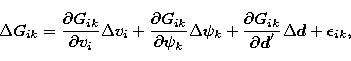$$\Delta G_{ik} = {\partial G_{ik}\over\partial v_i}\Delta v_i... ...over\partial {\vec{d}}^\prime}\Delta {\vec{d}} + \epsilon_{ik},$$ (1)

where G_ik is the grid coordinate of the star (the mean position on the grid during the observation as derived from its apparent position, the scan phase estimate and the reconstructed satellite attitude). $\psi_k$ is the along-scan attitude correction and ${\vec{d}}$ is the vector of instrument parameters. The very smooth motions of the satellite (except at times of thruster firings) allowed for the use of cubic splines to fit locally the corrections $\Delta \psi_k$ to the original star-mapper-based attitude reconstruction, and thus to reconstruct very precisely the abscissae along the great circle. However, the attitude corrections used the same abscissa data, and as a result there are correlations between the errors on the final abscissae and the attitude corrections. This propagated into correlations of abscissae errors for stars affected by the same attitude errors. Due to the two fields of view, abscissae errors for stars very close together on the sky, as well as for stars separated by 58 degrees (the basic angle) and multiples thereof, are found to be correlated (see Fig. 1). A preliminary study of these correlations was presented in Volume 3, Chapter 17. The correlations were re-investigated at a higher spatial resolution and taking into account the projection of the stellar separation to an abscissa difference. Also investigated was the influence of the length of the time interval covered by the data included in each great-circle reduction run. It was expected that correlations would be much stronger for short sets that for long sets. As the actual length of the data stretches was not available, the number of stars per great circle was used instead as an indicator of long and short sets. There were other aspects too, that affected the quality of the great-circle results, but these are difficult to reconstruct from the published data. They concern gaps in the data due to occultations (a major problem for great circles with small inclinations with respect to the ecliptic), and problems with the attitude reconstruction due to high background levels. Most of these problems reflect in individual abscissa accuracies.

Only stars with a standard 5-parameter solution were used in the determination of the correlations. On each great circle there are mostly between 900 and 2000 such stars (extremes run from 27 to 2110 stars for NDAC, and 295 to 2027 stars for FAST). Only in one situation were these correlations both significant and able to accumulate and affect a discussion of Hipparcos astrometric data: for stars in a small field (a few degrees diameter, like an open cluster or the Magellanic Clouds). For any other separation the correlation between measurements for a pair of stars seldom repeated themselves over the mission, and the cumulative effect was very small (stars at a separation of 180$^\circ$ also accumulated a correlation, but at that separation the correlations were rather small).

 

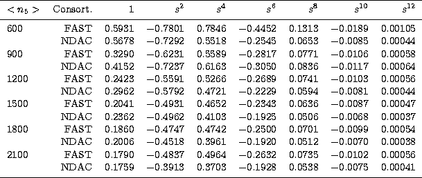
Table 1:   Functional representations of the correlation coefficients at short abscissa distances for different lengths of datasets. The lengths of the sets are indicated by n₅, which is the number of abscissae residuals accepted from 5-parameter solutions (Col. I in Table 2)

 

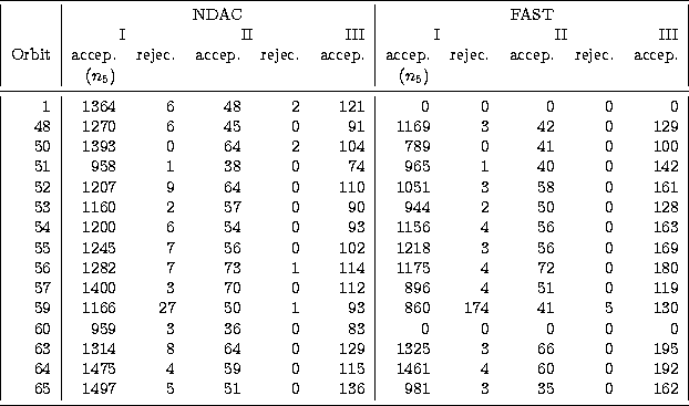
Table 2:   Numbers of abscissa residuals per orbit, split into three types of solutions: (I) type 5; (II) types 7, 9 and X; and (III) types C, V, O and -. In the first two cases the numbers of accepted and rejected residuals are given. For the third case only the number of abscissae was available. Only an extract of the Table is presented here. The full version is available in electronic form through the CDS

 

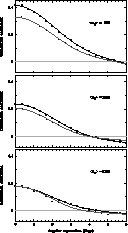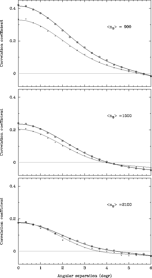
Figure 2:  The abscissa residuals correlation coefficient for small separations in data sets of different lengths. Top: short datasets; middle: medium length data sets; bottom: long datasets, as defined in Table 1. Crosses represent FAST data, open squares represent NDAC data. Also shown are the fits as given in Table 1

The strength of the correlations diminished when the time span covered by the data became longer. The increase in data decreased the degrees of freedom for the along-scan attitude improvements. The actual time span covered by each RGC is not recorded in the data files, but reflects in the number of stars included in each RGC. Figure 2 shows the correlations for short separations and for different ranges in dataset length. In particular for NDAC the increase in the correlations was strong for shorter datasets, reflecting one of the differences in the data reduction approach. The correlations were fitted with a polynomial in even powers of s, the abscissa separation measured in units of 4 degrees. The fits only cover the separation range 0 to 6 degrees, i.e. s ranging from 0 to 1.5. The results of those fits are summarized in Table 1. Table 2 (here only represented by an extract of the complete file, which is available electronically via the CDS) provides for each reference great circle the numbers of accepted and rejected abscissae. These data can also be used as an indicator of (the very few) generally unreliable reference great circles, by comparing the numbers of accepted and rejected observations. Section 6 shows how these correlations can be incorporated in a determination of a common proper motion or parallax for a group of stars with small separations on the sky.

The result of the great-circle reductions was a set of 2341 great circles. They cover a time-span of 2768 orbits or 1230 days. Not every great circle was reduced by both consortia. Due to a tape delivery problem that was detected too late, the NDAC reductions are not available for 4 RGCs towards the end of the mission, while in a few cases an RGC is missing in the FAST reductions due to problems with the data reductions. In most cases this concerned RGCs with small numbers of stars. Instrument parameters were not solved for when numbers of stars were low. They were interpolated from neighbouring, better determined solutions. For 2247 RGCs data is available from both consortia; for 15 RGCs data is only available from the FAST consortium; while for 79 RGCs data is only available from the NDAC consortium.

2.3 The sphere solution

 The main task for the sphere solution (Vol. 3, Chap. 16) was to establish reference zero points for all reference great circles, and to remove or calibrate any features left behind by the preceding processing. Although, as part of the sphere reconstruction, astrometric parameters were calculated, these are not the parameters presented in the catalogue. They were used to check the consistency between the solutions of the two consortia and to detect any grid-step ambiguities left over from the great-circle reduction. The result of the sphere reconstruction was, therefore, the original great-circle reduction data, with calibrated zero points and corrected systematic defects.

A comparison between the final Hipparcos and Tycho results seems to indicate the presence of grid-step ambiguities for 57 stars in the final catalogue (Vol. 4, Chap. 11). These stars can be solved for again by using the Tycho data as starting points and allowing corrections of multiples of $\pm 1.2074$ arcsec on some or all of the abscissae.

2.4 Merging and astrometric parameter determination

 Before any merging of data took place, the results from the two consortia had to be rotated to a common reference frame. This was done through the use of orthogonal rotations in positions and proper motions. As a first step, the formal errors on the FAST and NDAC data were investigated as functions of magnitude and quoted errors. The quoted errors were adjusted statistically to give the expected unit weight variances. Next, the correlation between the FAST and NDAC abscissa residuals were determined and applied. Astrometric solutions were made using the abscissae obtained by both consortia by incorporating the correlation coefficients. All solutions were tested for the necessity to allow a non-linear proper motion. In this process apparently outlying residuals or pairs of residuals were removed, and these can be recognized as such in the abscissa records. Solutions were accepted as either the standard 5-parameter model (two positional parameters, parallax and two proper motion parameters), the 7-parameter model (proper motion changing linearly with time) or in exceptional cases the 9-parameter model (proper motion changing quadratically with time). When none of these models provided an acceptable solution, and the star was not recognized as a double star, a so-called stochastic solution (indicated by ``X") was applied. In this solution, the 5-parameter model was implemented to the observed abscissae, but with the estimated errors on these abscissae artificially increased by adding quadratically ``cosmic noise'' until a satisfactory solution was obtained. The level of ``cosmic noise'' added is preserved in the DMSA part X, described in Sect. 2.3 of Volume 1. Any such solution has to be treated with great care. Likely interferences causing this ``cosmic noise'' are orbital motion (Bastian & Bernstein 1995; Bernstein 1997) and the presence of a planetary nebula. In all these cases the information provided in the Intermediate Astrometric Data file allows for a full reconstruction of the solution and its covariance matrix through the mechanism described in Sect. 3. Stars with solutions of type ``O" (orbital solutions) or ``-" (no astrometric solution) may also use the abscissae records. This is not the case for two other types of solutions, indicated with ``C'' and ``V". These represent a component solution and a ``variability induced mover'' respectively. The latter type stands for a small number of objects where duplicity was inferred by a photocentric motion caused by the variability of one of the components.

Finally, all results were transformed to the International Celestial Reference System (ICRS). This transformation was based mainly on very high accuracy radio positions and proper motions for a small set of radio stars (see Vol. 3, Chap. 18 and Kovalevsky et al. 1997).