Intensity profiles. The observed intensity profiles of the dust
continuum and the neutral radicals are shown in Fig. 5 (click here)
in double logarithmic presentation. Similar profiles for the molecular ions
are presented in Fig. 6 (click here). The continuum and molecular
band intensities I
are plotted as a function of the projected distance from the nucleus ![]() .
As there is no temporal variation apparent in the three data sets
(see Figs. 8 (click here) and 9 (click here)) the intensities
were plotted
without any distinction between the three data sets. To provide some spatial
resolution, the data were divided into four classes of profiles: sunward,
coma, tailward, and perpendicular to tail. Obviously
incorrect intensity values were not plotted.
.
As there is no temporal variation apparent in the three data sets
(see Figs. 8 (click here) and 9 (click here)) the intensities
were plotted
without any distinction between the three data sets. To provide some spatial
resolution, the data were divided into four classes of profiles: sunward,
coma, tailward, and perpendicular to tail. Obviously
incorrect intensity values were not plotted.
The figure panels 5 (click here)a-k and 6 (click here)a-o show in each row the same intensity values of one of the considered species in the form of black and grey dots. The grey, highlighted dots represent the selected values, i.e. the values belonging to the slit positions of the sunward, coma, and tailward areas in Fig. 5 (click here)a-k and the sunward, perpendicular to tail, and tailward areas in Fig. 6 (click here)a-o. The thin line is a fit to the highlighted, i.e. selected values. The selected slit positions are indicated for every profile in the panels 5 (click here)l-p and 6 (click here)p-t, respectively.
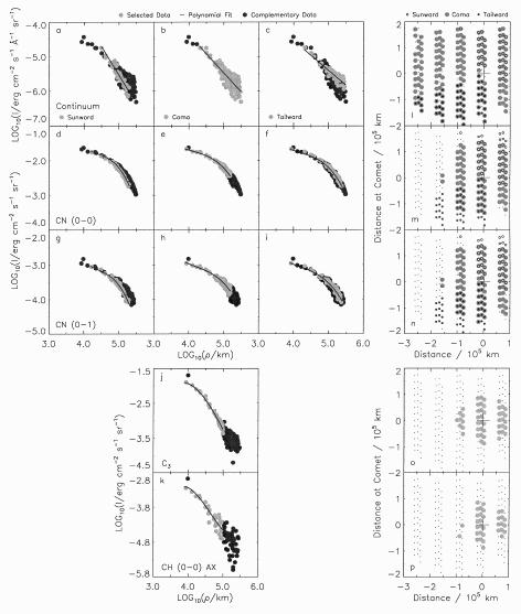
Figure 5: Radial intensity profiles of neutral coma constituents (a-k)
for different areas
of the coma (compare panels (l-p) with
Fig. 1 (click here))
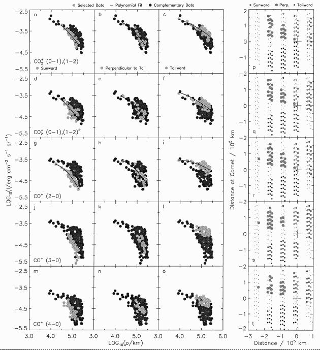
Figure 6: Radial intensity profiles of ionic coma constituents (a-o) for
different areas of
the coma (compare panels (p-t) with Fig. 1 (click here))
The intensity profiles of the dust continuum at 3650 Å
(Fig. 5 (click here)a-c) are expected to follow a ![]() law
(radial expansion of a particle cloud with constant speed). The deduced
gradient of the overall coma
profile (-1.1) is consistent with the expected value (-1) and with other
observations for P/Halley (e.g. Levasseur-Regourd et al. 1986;
Gammelgaard & Thomson 1988). The gradient of the tailward
profile (-.86) is consistent with the
law
(radial expansion of a particle cloud with constant speed). The deduced
gradient of the overall coma
profile (-1.1) is consistent with the expected value (-1) and with other
observations for P/Halley (e.g. Levasseur-Regourd et al. 1986;
Gammelgaard & Thomson 1988). The gradient of the tailward
profile (-.86) is consistent with the ![]() law, too, whereas the
sunward gradient (-1.6) shows a significant deviation. Jewitt &
Meech (1987) also found steeper gradients than -1 for P/Halley. As
an explanation Ellis & Neff (1992) considered temporal and
spatial variations in the dust production rate of P/Halley itself.
law, too, whereas the
sunward gradient (-1.6) shows a significant deviation. Jewitt &
Meech (1987) also found steeper gradients than -1 for P/Halley. As
an explanation Ellis & Neff (1992) considered temporal and
spatial variations in the dust production rate of P/Halley itself.
The strength of the continuum is given in Table 3 (click here) in units
of mean solar disc intensities (Allen 1973). The mean
solar disc intensity at 3650 Å is ![]() , i.e. the solar flux after Kurucz et al.
(1984) divided by the solid angle subtended by the sun at 1 AU
(Unsöld & Baschek 1988). For comparison of the dust
intensities with the literature the following equation (Jockers et al.
1993) was applied:
, i.e. the solar flux after Kurucz et al.
(1984) divided by the solid angle subtended by the sun at 1 AU
(Unsöld & Baschek 1988). For comparison of the dust
intensities with the literature the following equation (Jockers et al.
1993) was applied:
![]()
where p is the geometric albedo, ![]() the
phase angle of the comet, and
the
phase angle of the comet, and ![]() the phase function. In the
present paper the filling factor f is the local filling factor at the
projected distance
the phase function. In the
present paper the filling factor f is the local filling factor at the
projected distance ![]() from the cometary optocentre.
from the cometary optocentre.
![]() is expected to be a constant if
is expected to be a constant if
![]() varies with
varies with ![]() . The average of the table entries is
. The average of the table entries is
![]() . Note that the
Albedo-filling factor-distance product
. Note that the
Albedo-filling factor-distance product ![]() used by A'Hearn et al. (1984), and, e.g., Osip et al.
(1992) and Storrs et al. (1992) must be divided by 8 in
order to be comparable with our value (a factor of 4 arises from the
incorrect use of albedo by these authors and a further factor of 2 from the
fact that we refer to the local filling factor at the projected distance
used by A'Hearn et al. (1984), and, e.g., Osip et al.
(1992) and Storrs et al. (1992) must be divided by 8 in
order to be comparable with our value (a factor of 4 arises from the
incorrect use of albedo by these authors and a further factor of 2 from the
fact that we refer to the local filling factor at the projected distance ![]() and not to the filling factor averaged over a circular aperture with radius
and not to the filling factor averaged over a circular aperture with radius
![]() , see Jockers & Bonev 1997). For example,
the value of
, see Jockers & Bonev 1997). For example,
the value of ![]() provided by Osip et al. (1992) for comet Halley at the Giotto
encounter of
provided by Osip et al. (1992) for comet Halley at the Giotto
encounter of ![]() translates to a value of
translates to a value of
![]() .
.
It is not possible to directly compare our value with the (similar) value
of Osip et al. because we observed the comet at larger heliocentric distance
and a reduced phase angle as compared to the time of the Giotto encounter.
In addition,
Comet P/Halley showed brightness fluctuations with a period of 7.3 days
(Neckel & Münch 1987). Therefore, our data should only be
compared with results of publications referring to the same observation
time. Neckel & Münch (1987) have performed aperture
photometry of comet Halley. They provide four measurements between April
10.05 and 10.07, 1986, for four different circular apertures centered at the
nucleus. One filter (C) used by these authors peaked at 5250 Å with an
effective equivalent width of 100 Å. This wavelength band excluded
significant cometary emission lines and is close to the effective wavelength
of the V-band of the standard UBV filter system. Neckel & Münch
provide the cometary brightness measured in their continuum filter as V
magnitudes in the standard
Johnson UBV system. The solar magnitude mV equals -26.74 (Allen
1973). If we transfer fluxes to intensities by making use of the
apertures employed by Neckel and Münch (we did not use aperture 2 because
it was inconsistent with the other apertures) and the angular size of the
solar disk, and divide the resulting cometary intensity by two to transfer
the aperture-averaged intensity to the local intensity we obtain from
Eq. (4 (click here)) ![]() at
at ![]() , the
effective wavelength of the V-band. With Eq. (2 (click here)) we obtain at
3650 Å
, the
effective wavelength of the V-band. With Eq. (2 (click here)) we obtain at
3650 Å ![]() . This is
about the half of our value. This deviation is qualitatively confirmed by
a similar comparison (see below) for CN column densities.
. This is
about the half of our value. This deviation is qualitatively confirmed by
a similar comparison (see below) for CN column densities.
The profiles of the CN emissions (Figs. 5 (click here)d-i) indicate a nearly symmetrical cyanogen distribution. The small deviation between the sunward and tailward profiles arises from the acceleration effect of the solar radiation pressure on these particles. For P/Halley similar observations were made e.g. by Arpigny et al. (1986a) and Ellis & Neff (1992). Combi & Delsemme (1980) developed a model to determine the strength of that effect and published computed neutral profiles which are in excellent agreement with our CN profiles.
The ![]() intensity profile (Fig. 5 (click here)j) shows a strong
decrease toward the outer coma. The detectable
intensity profile (Fig. 5 (click here)j) shows a strong
decrease toward the outer coma. The detectable ![]() coma is too small to
reveal the effect of the radiation pressure. The CH profile
(Fig. 5 (click here)k) also does not show this effect, although
Wyckoff et al. (1988) reported a slight asymmetry between the
sunward and tailward parts of their CH profile for P/Halley.
coma is too small to
reveal the effect of the radiation pressure. The CH profile
(Fig. 5 (click here)k) also does not show this effect, although
Wyckoff et al. (1988) reported a slight asymmetry between the
sunward and tailward parts of their CH profile for P/Halley.
The ion profiles are plotted in Fig. 6 (click here). The
vertical extent of the cloud of data in these panels is much larger than for
the neutral emissions. This indicates the strong deviation of the plasma
cloud from spherical symmetry which is caused by the
interaction of the charged particles with the solar wind pushing the ions
tailward. The ![]() distribution is displayed in
Figs. 6 (click here)a-f and is in general
agreement with the variation of the
distribution is displayed in
Figs. 6 (click here)a-f and is in general
agreement with the variation of the ![]() emission around 2890 Å that
was found in sunward and tailward spectra of comet Bradfield 1979 X
(Festou et al. 1982). Both kinds of tailward profiles, the
normal one (Figs. 6 (click here)a-c) and that based on
consideration of the pseudocontinua (
emission around 2890 Å that
was found in sunward and tailward spectra of comet Bradfield 1979 X
(Festou et al. 1982). Both kinds of tailward profiles, the
normal one (Figs. 6 (click here)a-c) and that based on
consideration of the pseudocontinua (![]() ,
Figs. 6 (click here)d-f), suggest a local maximum in the ionic
coma content at about
,
Figs. 6 (click here)d-f), suggest a local maximum in the ionic
coma content at about ![]() . For the profiles with and
without pseudocontinuum the same polynomial fits were used, but with an
intensity offset. The profiles of the
. For the profiles with and
without pseudocontinuum the same polynomial fits were used, but with an
intensity offset. The profiles of the ![]() bands are shown in
Figs. 6 (click here)g-o. Only the (2-0) band could be used to
fit reliable profiles, because the (3-0) and (4-0) intensities near the
nucleus are probably still influenced by other emissions. The tailward
profiles of
bands are shown in
Figs. 6 (click here)g-o. Only the (2-0) band could be used to
fit reliable profiles, because the (3-0) and (4-0) intensities near the
nucleus are probably still influenced by other emissions. The tailward
profiles of ![]() also show the local ion maximum.
also show the local ion maximum.
Column density profiles. With Eq. (3 (click here)) the fitted molecular
intensity profiles were transformed to column density profiles which are shown
in Figs. 7 (click here)a-c. The profiles of CN (0-0)
and (0-1) are in good agreement for the coma and the tailward areas,
respectively, only the sunward profiles show a slight offset. The relative
error of all CN column densities is found to be not worse than about 10%.
The column densities were averaged (Table 3 (click here)) and the resulting
mean profile was quantitatively compared with the CN profile of P/Halley for
April 10.40, 1986, that was published by Combi et al. (1994).
Our column densities are larger by a factor of about ![]() than the referenced profile.
This deviation is in qualitative agreement with the analogous factor of 2
which was deduced (see above) from a comparison for dust continuum
intensities.
than the referenced profile.
This deviation is in qualitative agreement with the analogous factor of 2
which was deduced (see above) from a comparison for dust continuum
intensities.
![]()
Figure 7: Radial column density profiles of observed coma
constituents a-c)
for different areas of the coma
For the ![]() and CH radicals only coma profiles could be fitted. Both profiles
show a more rapid decrease with increasing distance from nucleus than in the
case of CN. For
and CH radicals only coma profiles could be fitted. Both profiles
show a more rapid decrease with increasing distance from nucleus than in the
case of CN. For ![]() this is in agreement with Goraya et al.
(1988), Hu et al. (1988), and Ellis & Neff
(1992). The
this is in agreement with Goraya et al.
(1988), Hu et al. (1988), and Ellis & Neff
(1992). The ![]() profile is only slightly steeper than the CH
profile. Figures 7 (click here)a-c indicate the
coma extension at a constant column density: the CN coma is the largest one
followed by the
profile is only slightly steeper than the CH
profile. Figures 7 (click here)a-c indicate the
coma extension at a constant column density: the CN coma is the largest one
followed by the ![]() and CH comae. Mitchell et al. (1981)
created a model to predict particle density profiles for several neutral
coma constituents. Their calculated abundances for CN,
and CH comae. Mitchell et al. (1981)
created a model to predict particle density profiles for several neutral
coma constituents. Their calculated abundances for CN, ![]() , and CH,
are in good agreement with our observed profiles, whereas the gradients of
their profiles do not describe the present profiles well.
, and CH,
are in good agreement with our observed profiles, whereas the gradients of
their profiles do not describe the present profiles well.
For ![]() two sets of profiles, connected by a shaded area, are shown in
Fig. 7 (click here). The upper profiles were directly
deduced from the overall intensity in the
two sets of profiles, connected by a shaded area, are shown in
Fig. 7 (click here). The upper profiles were directly
deduced from the overall intensity in the ![]() integration range, whereas
the lower profiles take an additional pseudocontinuum into account. As mentioned
above, the two profiles differ only by a constant, which gives credibility
to the relative trend. The
tailward profile of
integration range, whereas
the lower profiles take an additional pseudocontinuum into account. As mentioned
above, the two profiles differ only by a constant, which gives credibility
to the relative trend. The
tailward profile of ![]() shows a steeper gradient than the corresponding
shows a steeper gradient than the corresponding
![]() profile; this is consistent with observations of comet
West 1976 VI (A'Hearn & Feldman 1980). The
sunward profiles do not reveal significant differences in the decrease of
the two species. The profile perpendicular to the tail shows a
slightly larger decrease of
profile; this is consistent with observations of comet
West 1976 VI (A'Hearn & Feldman 1980). The
sunward profiles do not reveal significant differences in the decrease of
the two species. The profile perpendicular to the tail shows a
slightly larger decrease of ![]() as compared to
as compared to ![]() .
Wegmann et al. (1987) have developed a three-dimensional model
to determine particle density profiles for different ionic coma
constituents. This model confirms the steeper gradients perpendicular to the
tail but in contrast to our observations the tailward gradient of
.
Wegmann et al. (1987) have developed a three-dimensional model
to determine particle density profiles for different ionic coma
constituents. This model confirms the steeper gradients perpendicular to the
tail but in contrast to our observations the tailward gradient of ![]() and
and ![]() is nearly equal. Because all ions move with the same
velocity nearly parallel to the tail axis, the steeper gradient
perpendicular to the tail indicates a less extended source region for
is nearly equal. Because all ions move with the same
velocity nearly parallel to the tail axis, the steeper gradient
perpendicular to the tail indicates a less extended source region for ![]() . The observed steeper gradient in tailward direction could be
caused by a destruction process of
. The observed steeper gradient in tailward direction could be
caused by a destruction process of ![]() , which is not implemented in
the model, like perhaps photodissociation. This additional process would
lead to a shorter
, which is not implemented in
the model, like perhaps photodissociation. This additional process would
lead to a shorter ![]() mean life time as compared to
mean life time as compared to ![]() .
.
The ion profiles in Fig. 7 (click here) indicate, even if a
![]() pseudocontinuum is considered, that
pseudocontinuum is considered, that ![]() is less abundant than
is less abundant than
![]() . This conclusion is inconsistent with observations for comet
Giacobini-Zinner by A'Hearn et al. (1986) which found a column
density for
. This conclusion is inconsistent with observations for comet
Giacobini-Zinner by A'Hearn et al. (1986) which found a column
density for ![]() (2188 Å) that might be about a magnitude higher
than their value for
(2188 Å) that might be about a magnitude higher
than their value for ![]() (2888 Å). Supplementary, Krankowsky
(1991) reported a CO production rate for P/Halley that is larger than
that of
(2888 Å). Supplementary, Krankowsky
(1991) reported a CO production rate for P/Halley that is larger than
that of ![]() . The photochemical lifetime of these neutral molecules,
the most important parents for
. The photochemical lifetime of these neutral molecules,
the most important parents for ![]() and
and ![]() , is similar.
Therefore their abundance ratio is expected to be roughly transferred by the
photoionization process to their daughter molecules. Also the models of Ip
(1981) and Wegmann et al. (1987) predict larger particle
densities for
, is similar.
Therefore their abundance ratio is expected to be roughly transferred by the
photoionization process to their daughter molecules. Also the models of Ip
(1981) and Wegmann et al. (1987) predict larger particle
densities for ![]() than for
than for ![]() . The inconsistency between
these models and our data may be explained by the performed intensity
calibration: in the
. The inconsistency between
these models and our data may be explained by the performed intensity
calibration: in the ![]() wavelength range the response function had
to be extrapolated (see Fig. 3 (click here)b). After all, it is probably
necessary to consider a pseudocontinuum for
wavelength range the response function had
to be extrapolated (see Fig. 3 (click here)b). After all, it is probably
necessary to consider a pseudocontinuum for ![]() . Additionally, the
. Additionally, the
![]() column densities depend on preliminary fluorescence emission
rates.
column densities depend on preliminary fluorescence emission
rates.
There is no doubt that the Haser (1957) model is too simple to
adequately describe the distribution of neutral radicals in a cometary coma
(see Festou et al. 1993, Sect. 4.3.2), but it is still widely
used. Therefore, in order to compare our data set with others we have
determined Haser scalelengths from our profiles. The model
was implemented using equations for the Bessel functions of Abramowitz
& Stegun (1984). For the determination of the parent and daughter
scale lengths, p and d, their parameter space was searched for those
values leading to an absolute minimum of the ![]() function which was
defined in the usual way by comparing the normalized observed coma profile
with the modeled one. The results are given in Table 4 (click here). For
function which was
defined in the usual way by comparing the normalized observed coma profile
with the modeled one. The results are given in Table 4 (click here). For
![]() and CH, respectively, this method yielded a parameter pair that
fits the observed profiles best, whereas the CN profiles could be fitted
with several pairs of scale lengths (see also Cochran 1985).
This is caused by the huge extent of the CN coma compared even with our
field of
and CH, respectively, this method yielded a parameter pair that
fits the observed profiles best, whereas the CN profiles could be fitted
with several pairs of scale lengths (see also Cochran 1985).
This is caused by the huge extent of the CN coma compared even with our
field of ![]() diameter. Therefore, a nominal
value for the CN daughter scale length was taken from A'Hearn
(1982). Meredith et al. (1992) present CN parent scales
for a number of comets. These authors show that a scaling of the scale
length according to the square heliocentric distance (as was done by us)
frequently is not a good fit to their data. When this is taken into account
our parent scale length agrees well with their values for minimum solar
activity conditions (comet Halley).
diameter. Therefore, a nominal
value for the CN daughter scale length was taken from A'Hearn
(1982). Meredith et al. (1992) present CN parent scales
for a number of comets. These authors show that a scaling of the scale
length according to the square heliocentric distance (as was done by us)
frequently is not a good fit to their data. When this is taken into account
our parent scale length agrees well with their values for minimum solar
activity conditions (comet Halley).
|
Molecule | p | d | Q/v | |
|
| (km) | (km) | (km-1) | |
|
CN (0-0) | | |
| |
| (0-1) | | |
| |
|
| | |
| |
| CH | | |
| |
|
|
Using the obtained scale lengths and the method of Newburn & Spinrad
(1984) the quantity Q/v, i.e. the production rate divided by the
neutral radial outflow velocity, was determined for each radical. Assuming
![]() Q/v can easily be transformed to a production rate. The given
rmse represents the goodness of the fit.
Q/v can easily be transformed to a production rate. The given
rmse represents the goodness of the fit.