Intensity and column density maps. The distributions of the dust continuum and the molecular species are shown as contour plots in Figs. 8 (click here) and 9 (click here). These two-dimensional maps present the measured continuum intensities and column densities in logarithmic scale with respect to their spatial resolution (compare Fig. 1 (click here)). Generally, the distributions decrease from a peak near the cometary nucleus (+) towards the outer coma. In the maps the shape of the contour lines strongly depends on single values of the nonuniformly distributed data points (intensity or column density values and their corresponding slit positions). Therefore, some strongly deviating data points could not be used for properly interpolating the maps. In the case of the data sets A and C the cometary nucleus is covered quite well with a slit column of the slit plate (Fig. 1 (click here)), and therefore, the centers of the interpolated distributions are very close to the nucleus. For data set B this condition is not met, and the centers of the deduced distributions differ from the position of the nucleus. The neutral distributions do not show a variation with time. Therefore, the three corresponding maps of each considered neutral coma constituent were superposed to create additional maps with a higher spatial resolution (Figs. 8 (click here)p-t).
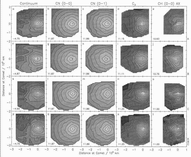
Figure 8: Celestial plane projection of the distribution of
neutral coma constituents for the data sets A (a-e), B (f-j), C
(k-o), and their superposition ABC (p-t). The values of the
innermost contour lines are given in ![]() ) in the case of the dust continuum at 3650
Å, and in
) in the case of the dust continuum at 3650
Å, and in ![]() ) in the case of the radicals; the
contour level decrement is always
) in the case of the radicals; the
contour level decrement is always ![]()
The dust coma has a nearly symmetrical distribution within a projected radius
of approximately ![]() which is best seen in the superposed dust
map. The detectable dust coma was well covered by the large field of view of
the focal reducer, but only the innermost part of the dust tail, that had a
length of several degrees at observation time (Ozeki 1986;
Lamy et al. 1987), appears in the lower left part of the maps.
which is best seen in the superposed dust
map. The detectable dust coma was well covered by the large field of view of
the focal reducer, but only the innermost part of the dust tail, that had a
length of several degrees at observation time (Ozeki 1986;
Lamy et al. 1987), appears in the lower left part of the maps.
As expected from the CN profiles, the cyanogen maps also reveal quite a
symmetrical CN coma with a slight deformation caused by the effect of the solar
radiation pressure (Sect. 5.1 (click here)). The contour lines of the CN
(0-1) maps are not as circular as those of the CN (0-0) maps because the
related band intensities are smaller and have a larger relative error, but the
general agreement is very good. Kidger et al. (1987) also
published maps for both CN emissions. The ![]() coma is found to have a
symmetrical particle distribution. Kidger et al. (1987) also
found no significant deviation from spherical symmetry. In our maps, the
shape of the contour lines in the lower left part may be due to an
unidentified ion emission contaminating the
coma is found to have a
symmetrical particle distribution. Kidger et al. (1987) also
found no significant deviation from spherical symmetry. In our maps, the
shape of the contour lines in the lower left part may be due to an
unidentified ion emission contaminating the ![]() emission. The CH maps
of the three data sets are not very similar. Therefore, the strength of the
CH emission mark a lower intensity limit: weaker emissions could not be used
for interpolating reliable profiles and maps. The CH emission in the spectra
of the left slit column were too weak to be measured. The superposed CH map
reveals a detectable CH coma that is slightly smaller than the
emission. The CH maps
of the three data sets are not very similar. Therefore, the strength of the
CH emission mark a lower intensity limit: weaker emissions could not be used
for interpolating reliable profiles and maps. The CH emission in the spectra
of the left slit column were too weak to be measured. The superposed CH map
reveals a detectable CH coma that is slightly smaller than the ![]() coma. The presented maps for CN (0-0),
coma. The presented maps for CN (0-0), ![]() , and CH, are in agreement
with the observations by Kidger et al. (1987).
, and CH, are in agreement
with the observations by Kidger et al. (1987).
The distributions of ![]() and
and ![]() show a significant deviation from
spherical symmetry that is caused by the interaction of these particles with
the solar wind. The decrease towards the sun is always stronger than that in
tailward direction, and the tailward gradient of
show a significant deviation from
spherical symmetry that is caused by the interaction of these particles with
the solar wind. The decrease towards the sun is always stronger than that in
tailward direction, and the tailward gradient of ![]() is found to be less
steep than that of
is found to be less
steep than that of ![]() . Close to the nucleus, the ion maps are much
flatter than the maps of the neutral species and the dust, and show a plateau
extending from the nucleus into the tail. A similar flat distribution of the
. Close to the nucleus, the ion maps are much
flatter than the maps of the neutral species and the dust, and show a plateau
extending from the nucleus into the tail. A similar flat distribution of the
![]() ion has been observed in comet Austin by Bonev & Jockers
(1994). The ion maps which are based on an intensity integration that
considered a pseudocontinuum (Figs. 9 (click here)b-e, g-j, l-o)
suggest the existence of plasma clouds in the tail. This is supported by
Jockers et al. (1987) which published a time series of direct
filter images of comet P/Halley for April 11, 1986, in the light of
ion has been observed in comet Austin by Bonev & Jockers
(1994). The ion maps which are based on an intensity integration that
considered a pseudocontinuum (Figs. 9 (click here)b-e, g-j, l-o)
suggest the existence of plasma clouds in the tail. This is supported by
Jockers et al. (1987) which published a time series of direct
filter images of comet P/Halley for April 11, 1986, in the light of ![]() (3674 Å) and
(3674 Å) and ![]() (4252 Å) that both show the
ejection of a plasma cloud. The modeled column density maps for
(4252 Å) that both show the
ejection of a plasma cloud. The modeled column density maps for ![]() and
and ![]() by Wegmann et al. (1987) are consistent with
our large scale distributions with the exception of the tailward gradient
observed for
by Wegmann et al. (1987) are consistent with
our large scale distributions with the exception of the tailward gradient
observed for ![]() .
.
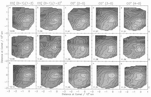
Figure 9: Celestial plane
projection of the distribution of ionic coma constituents for the data sets A
(a-e), B (f-j), and C (k-o). The values of the innermost
contour lines are given in ![]() ); the contour level
decrement is equal to 0.1505
); the contour level
decrement is equal to 0.1505