The plates were digitized in May 1992, at ESO-Headquarters in Garching,
Germany, using a PDS 1010A microdensitometer (Eccles et al.
1983) with an aperture of ![]() . The direct
filter images were scanned in
. The direct
filter images were scanned in ![]() steps in each direction. In
the scans of the multislit spectra the steps in the direction perpendicular
to the slits was reduced to
steps in each direction. In
the scans of the multislit spectra the steps in the direction perpendicular
to the slits was reduced to ![]() , i.e. the spectra were
oversampled in dispersion direction.
, i.e. the spectra were
oversampled in dispersion direction.
Characteristic curve. The characteristic curve of the plates (see Eccles et al. 1983) was determined by a sensitometer calibration. The calibration plate was exposed 600 s using the ESO tube spot sensitometer with a BG18/OG515 filter combination approximating the colour of the phosphor output window of the image intensifier.
Alignment of images. One direct image with the slit pattern superimposed on the comet images was rotated to align the slits to the vertical image axis (see Fig. 1 (click here)). Then all images were adjusted relative to each other by making use of the fixed pattern of the small intensifier spots, existing on all plates. The accuracy of this reduction step in terms of spectral resolution was about 1 Å.
![]()
Figure 2: Comparison of corresponding pixel values in processed images F167,
F168, and F169 with 30, 10, and 3 min exposure
Adjustment of exposure times. The relative intensities of the 3 and
30 min. exposures of each data set were adjusted to the intensities of the 10
min. exposure. The relevant exposure times (Table 1 (click here)) gave
adjustment factors of ![]() and
and ![]() , respectively.
For verification, the intensity values of corresponding pixels in the
spectra images were directly compared. Only pixels belonging to a spectrum
and the reliable intensity interval of the characteristic curve were
selected, pixels of the plate background and of detector blemishes were
rejected. For data set B the result is shown in Fig. 2 (click here).
About 105 pixel values of the images F167 and F169 are plotted against
the value of the corresponding pixels in image F168. In
Fig. 2 (click here) the slopes of the straight lines are the exposure
time ratios. The deviations from linearity are probably caused by the
characteristic curve underestimating the values of the higher intensities.
Furthermore, the different airmasses (Table 1 (click here)) in combination
with the coefficient of extinction may result in some wavelength dependence
of the factors. Therefore, instead of the exposure time ratios empirical
factors (Table 1 (click here)) deduced from the pixel comparison itself
were applied to the images. Figure 2 (click here) indicates that,
after adjusting the exposure times, image F167 was the more important source
for low intensities while F169 was more important for high intensities,
i.e. the dynamic intensity range of image F168 was effectively enlarged.
, respectively.
For verification, the intensity values of corresponding pixels in the
spectra images were directly compared. Only pixels belonging to a spectrum
and the reliable intensity interval of the characteristic curve were
selected, pixels of the plate background and of detector blemishes were
rejected. For data set B the result is shown in Fig. 2 (click here).
About 105 pixel values of the images F167 and F169 are plotted against
the value of the corresponding pixels in image F168. In
Fig. 2 (click here) the slopes of the straight lines are the exposure
time ratios. The deviations from linearity are probably caused by the
characteristic curve underestimating the values of the higher intensities.
Furthermore, the different airmasses (Table 1 (click here)) in combination
with the coefficient of extinction may result in some wavelength dependence
of the factors. Therefore, instead of the exposure time ratios empirical
factors (Table 1 (click here)) deduced from the pixel comparison itself
were applied to the images. Figure 2 (click here) indicates that,
after adjusting the exposure times, image F167 was the more important source
for low intensities while F169 was more important for high intensities,
i.e. the dynamic intensity range of image F168 was effectively enlarged.
Average of images. The averaged multislit spectra image A of a data
set was calculated from the three corresponding spectra images I1, I2,
and I3, using the equation
![]()
The weights ![]() were formed out of mask images
were formed out of mask images ![]() and
error images
and
error images ![]() which were created for every spectrum image
which were created for every spectrum image
![]() . The pixel values of the mask images were set to 1 and 0,
respectively, depending on wether the related pixels in the spectra images
contained useful spectral information or not. This way, pixel values
contaminated by background stars, the fixed pattern of the intensifier
spots, scratches on some plates, or limitations caused by the characteristic
curve, were marked with 0. The pixel values in the error images were
estimated errors of the corresponding pixel values in the spectra images.
These error images were created just after applying the characteristic curve
to the digitized images, and were processed in the same way.
. The pixel values of the mask images were set to 1 and 0,
respectively, depending on wether the related pixels in the spectra images
contained useful spectral information or not. This way, pixel values
contaminated by background stars, the fixed pattern of the intensifier
spots, scratches on some plates, or limitations caused by the characteristic
curve, were marked with 0. The pixel values in the error images were
estimated errors of the corresponding pixel values in the spectra images.
These error images were created just after applying the characteristic curve
to the digitized images, and were processed in the same way.
Figure 3: Steps in the data reduction of a cometary head spectrum (marked by an
arrow in Fig. 1 (click here)): Extraction a), calibration b), and
approximation of the dust continuum c)
Extraction of spectra. The skew between the slit direction and the
dispersion in the averaged multislit spectra images was removed by shearing
these images parallel to the slits by an angle of ![]() .
One-dimensional spectra were then extracted by averaging up to 15 pixel values
in slit direction. In Fig. 3 (click here)a an extracted cometary head
spectrum is shown. The related slit position is marked in
Fig. 1 (click here) with an arrow.
.
One-dimensional spectra were then extracted by averaging up to 15 pixel values
in slit direction. In Fig. 3 (click here)a an extracted cometary head
spectrum is shown. The related slit position is marked in
Fig. 1 (click here) with an arrow.
Subtraction of plate background. To correct for the large-scale intensifier background on the plates the nearby emission-free area surrounding each spectrum was used to approximate the individual background for that spectrum. In Fig. 3 (click here)a this approximation is shown as a thin line below the spectrum.
Wavelength calibration. The wavelength calibration was done by
identifying spectral emission features of known wavelengths in the cometary
spectra and comparing them with maximum intensity wavelengths
published by Swings & Haser (1956). The reciprocal linear
dispersion of the five spectra columns of data set C for example resulted in
95.2, 94.1, 93.5, 92.1, and ![]() , respectively. The
wavelength co-ordinate was rectified with a polynomial of first degree. The
NGC 6302 spectrum was extracted the same way as the Halley spectra, but for
the wavelength calibration the publications of Aller & Czyzak
(1978) and Aller et al. (1981) were used.
, respectively. The
wavelength co-ordinate was rectified with a polynomial of first degree. The
NGC 6302 spectrum was extracted the same way as the Halley spectra, but for
the wavelength calibration the publications of Aller & Czyzak
(1978) and Aller et al. (1981) were used.
Intensity calibration. The extracted spectra were corrected for
extinction using the computed airmasses of the the plates with 600 s exposure
(Table 1 (click here)) and the nominal ESO coefficient of extinction
published by Danks (1983). The intensities of the spectra were
normalized to 1 s. To determine the response function of the spectra, the
relative line intensities of eight NGC 6302 emission features were
integrated and compared to known absolute line intensities
(Fig. 3 (click here)b). For this purpose, relative intensities from Oliver
& Aller (1969), Aller & Czyzak (1978), and Aller
et al. (1981), were calibrated using absolute intensities for ![]() ,
, ![]() , and [OIII], which were deduced from
Danziger et al. (1973). The response function was approximated
by a Gaussian curve. The calibrated example spectrum is shown in
Fig. 3 (click here)c.
, and [OIII], which were deduced from
Danziger et al. (1973). The response function was approximated
by a Gaussian curve. The calibrated example spectrum is shown in
Fig. 3 (click here)c.
Dust continuum. In the reduced spectra a contribution
of the solar spectrum is visible which is backscattered from the cometary
dust grains. In order to model this dust continuum and to create a solar
spectrum ![]() with the resolution of the
instrument, the FWHM of the cometary spectra (5.2 Å) was
determined from the well resolved emission lines of the NGC 6302 spectrum.
Then the solar spectrum published by
Kurucz et al. (1984) was convolved with the corresponding
Gaussian curve to adjust the spectral resolution. The reddening of the dust
continuum of P/Halley with respect to the solar spectrum was considered by
applying the following equation of Werner et al. (1989), which
is in accordance with the color values presented by Meech & Jewitt
(1987) and Thomas & Keller (1989):
with the resolution of the
instrument, the FWHM of the cometary spectra (5.2 Å) was
determined from the well resolved emission lines of the NGC 6302 spectrum.
Then the solar spectrum published by
Kurucz et al. (1984) was convolved with the corresponding
Gaussian curve to adjust the spectral resolution. The reddening of the dust
continuum of P/Halley with respect to the solar spectrum was considered by
applying the following equation of Werner et al. (1989), which
is in accordance with the color values presented by Meech & Jewitt
(1987) and Thomas & Keller (1989):
![]()
The resulting spectrum was adjusted to the cometary spectra in a way, that
after its subtraction a maximum continuum contribution was removed without
leading to negative intensities in the wavelength range between 3750 and 4350
Å. The strength of each approximated dust continuum was then measured in
the continuum window at 3650 Å. An adjusted continuum is shown in
Fig. 3 (click here)c. Even around 3600 Å the approximation still fits the
dust continuum very well.
Molecular bands. To identify the emission features in the cometary
spectra they were compared with theoretical and laboratory wavelengths and
observed spectra (Gerö 1941; Mrozowski 1947a,b;
Swings & Haser 1956; Gausset et al. 1965;
Brocklehurst et al. 1972; McCallum & Nicholls
1972; Zucconi & Festou 1985; Arpigny et al.
1986a,b; Magnani & A'Hearn 1986; Jockers
et al. 1987; Wyckoff & Theobald 1989; Valk et al.
1992; Kim & A'Hearn 1993, pers. communication; Lutz et al.
1993). The extracted spectra show a large number of cometary
emissions of different sources, but for the present paper the stronger and
sufficiently resolved emissions rather than tentative identifications were
considered. The selected emissions with their peak wavelengths and
integration intervals are listed in Table 2 (click here) and marked in
Fig. 4 (click here). If possible, we did not rely on the continuum
subtraction described in the previous paragraph, but interpolated a
so-called pseudocontinuum between long and short wavelength side of the
molecular emission. In the case of ![]() the band intensity was
integrated with and without considering a pseudocontinuum. The emission of
the band intensity was
integrated with and without considering a pseudocontinuum. The emission of
![]() around 4050 Å is mainly contaminated by the
around 4050 Å is mainly contaminated by the ![]() (3-0) emission, and therefore its integration range was reduced to exclude
this contamination. The integrated
(3-0) emission, and therefore its integration range was reduced to exclude
this contamination. The integrated ![]() intensities were multiplied
with 2.12 to adjust for the whole
intensities were multiplied
with 2.12 to adjust for the whole ![]() band. This factor was deduced
from the strongest head spectrum where the
band. This factor was deduced
from the strongest head spectrum where the ![]() (3-0) contamination
could be neglected. No emissions of the night sky were found in the spectra.
(3-0) contamination
could be neglected. No emissions of the night sky were found in the spectra.
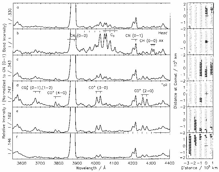
Figure 4: Synopsis of spectra a-f) averaged over different areas of
the cometary coma (compare panels g-l) with
Fig. 1 (click here))
The integrated molecular band intensities I were transformed to column
densities N using the fluorescence emission rates g listed in
Table 2 (click here) and the equation
![]()
(see Lutz et al. 1993). The used emission rate for ![]() is preliminary and may be revised in the future.
is preliminary and may be revised in the future.