2 Modeling approach

The modeling approach is based on the incoherent space-invariant imaging equation describing the imaging of an incoherently radiating object through an optical system:

$$i^{Pol}(\vec{x}) = o^{Pol}(\vec{x}) \ast PSF^{Pol}(\vec{x}); Pol \equiv s,p$$ (1)

where $i^{Pol}(\vec{x})$ and $o^{Pol}(\vec{x})$ denote the intensity distributions of the image and object respectively, $PSF^{Pol}(\vec{x})$ the point spread function, $\vec{x}$ a two dimensional vector in image space. The equation holds for the two uncorrelated orthogonal source polarizations of the naturally polarized source specified by the superscript $Pol \equiv s,p$. In the spatial frequency domain the convolution ("$\ast$'') in Eq.(1) becomes a multiplication:

$$I^{Pol}(\vec{u}) = O^{Pol}(\vec{u})\ OTF^{Pol}(\vec{u}); Pol \equiv s,p$$ (2)

with $I^{Pol}(\vec{u})$, $O^{Pol}(\vec{u})$, $OTF^{Pol}(\vec{u})$ being the Fourier transforms of $i^{Pol}(\vec{x})$, $o^{Pol}(\vec{x})$, $PSF^{Pol}(\vec{x})$. $\vec{u}$ is a two dimensional vector in Fourier space. The components of $\vec{u}$ are usually called u and v, spanning the uv-plane. $O^{Pol}(\vec{u})$ is the object complex visibility of the object for each source polarization ( $Pol \equiv s,p$). $OTF^{Pol}(\vec{u})$ is the optical transfer function (OTF). The OTF is the normalized autocorrelation of the electric field distribution in the exit pupil ("pupil function'', see Eq.8). The modulus of the optical transfer function is called the modulation transfer function (MTF). Equation(2) is the basis for all our modeling algorithms. The calculation of $O^{Pol}(\vec{u})$ and $OTF^{Pol}(\vec{u})$ enables us to obtain the fringe pattern as seen by an optical interferometer. Equations (1) and (2) hold for a single wavelength $\lambda$ ("monochromatic light'').

Figure 1: The modeling approach is based on an optomechanical End-to-End model computing the dynamic instrument response to a point source and a beam combination/imaging model which simulates the imaging of an extended object using a Fourier optical formalism. Note that the peaks in the entrance OTF and in the two exit OTFs have different spacings In case of multiaxial beam combination the three peaks of the exit OTF are not necessarily adjacent to each other. The multiplication of the object complex visibility and the exit OTF is done after shifting the selected visibility regions onto the three OTF peaks appropriately. The interferometric image in the coaxial mode has to be modulated in time to retrieve any object visibility

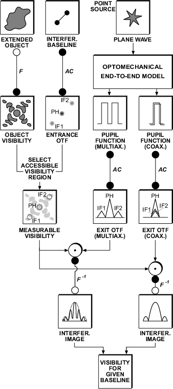
Figure1 illustrates the basic modeling approach. As response to a point source an optomechanical End-to-End model computes the time-dependent electric field distribution ("pupil function'') in the exit pupils of the different interferometer arms (at the entrance of the beam combiner). We assume observation of the source in a narrow spectral band (bandwidth $\Delta\lambda \ll$ center wavelength $\lambda$) ("quasimonochromatic approach''). The OTF which in general is wavelength-dependent is computed for the center wavelength of the quasimonochromatic band. The End-to-End model includes models for mechanical structure, control system, environmental disturbances and - as core part - an optical model based on a hybrid ray tracing and diffraction propagation code (Denise & Koehler 1998; Wilhelm et al. 1998; Wilhelm & Johann 1999). The output of the optomechanical model serves as input to a separate Fourier optical model which computes the time-dependent optical transfer function at the exit pupil ("exit OTF'') for coaxial ("pupil-plane'') and multiaxial ("image-plane'') beam combination (Schöller et al. 1998). The exit OTF combines the interferometer OTF and atmospheric effects in a single quantity. For a given baseline $\vec{B}$ (projected perpendicular to the direction of observation) the accessible regions of the object visibility in the spatial frequency domain are determined by the "non-zero'' domains of the "entrance OTF'' which itself is given by the autocorrelation (denoted by "AC'' in Fig.1) of the electric field distribution in the entrance pupil corresponding to the interferometer baseline ("entrance baseline'').

Both, exit and entrance OTF consist of three cone-shaped peaks in the spatial frequency plane ("uv-plane''): a central "photometric peak'' (denoted by "PH'' in Fig.1) around zero spatial frequency $\vec{u} = 0$ and two "interferometric peaks'' (denoted by "IF1'' and "IF2'' in Fig.1), symmetric with respect to the origin of the spatial frequency plane. The photometric peak holds only the information of the single apertures, including the total flux. The interferometric peaks hold the interferometric signal, which results from the coherent superposition of the beams related to the two interferometer arms. In the case of a "source visibility'' of 1 the interferometric peaks reach their maximum height equal to half the height of the photometric peak, leading to maximum fringe contrast. The interferometric peaks are located at the spatial frequencies corresponding to the entrance and exit baseline, respectively ( $\vec{u} = \pm \vec{B}/\lambda$ for entrance OTF, $\vec{u} = \pm \vec{B}^{\prime}/\lambda$ for exit OTF). The exit baseline $\vec{B}^{\prime}$ is given by the distance of the two interferometric beams before superposition (in the beam combiner). In case of coaxial beam combination the exit baseline is zero ( $\vec{B}^{\prime} = {\bf0}$). For a Fizeau-type interferometer which always uses multiaxial beam combination the entrance and exit baseline coincide ( $\vec{B}^{\prime} = \vec{B}$, in all three coordinates (u,v,w)), i.e. there is no difference between entrance and exit OTF. On the other hand, in case of a Michelson-type interferometer the exit baseline typically is much shorter than the entrance baseline ( $\left\vert\vec{B}^{\prime}\right\vert \ll \left\vert\vec{B}\right\vert$), hence entrance and exit OTF are different.

The interferometric image for the selected baseline is obtained as follows: The three distinct measurable parts of the object visibility map are multiplied with the corresponding peaks of the exit OTF ("IF1'', "PH'' and "IF2'') (Tallon & Tallon-Bosc 1992). Inverse Fourier transform of the resulting visibility map yields the interferometric image. For both beam combination modes the envelope of the image is given by the diffraction pattern corresponding to the individual pupils before their combination. While in the multiaxial mode spatial fringes are directly visible in the image a detection in the coaxial mode requires a modulation of the optical path in one interferometer arm to create a temporal fringe pattern. The spacing of the fringes is determined by the exit baseline $\vec{B}^{\prime}$ or the optical path modulation function for multiaxial or coaxial beam combination, respectively. For both beam combination schemes the fringe contrast is determined by the source visibility map sampled at the spatial frequencies $\pm \vec{B}/\lambda$. Various algorithms exist for estimating the complex visibility (contrast and phase of the fringe pattern) from a measured spatial or temporal fringe pattern.

The regrouping of the pupils in a Michelson interferometer results in a PSF which is changing over the field-of-view. Tallon & Tallon-Bosc (1992) describe the object-image relationship for a Michelson interferometer in the monochromatic case. The description of a Michelson interferometer by the incoherent space invariant imaging equation is an approximation which is only correct for a sufficiently small interferometric field-of-view. Outside of this interferometric field-of-view the fringe contrast is deteriorated until there are no fringes anymore. The object intensity distribution has to be convoluted with a field dependent PSF to describe the image intensity distribution. This PSF is not changing in the direction perpendicular to the baseline.

In our simulations we are still using the description by the incoherent space invariant imaging equation, limiting ourselves to a field-of-view with the size of an Airy disk, corresponding to a single subaperture of the interferometer. This is a valid way to describe observations with an interferometer, if the instruments use a spatial filter, thus limiting their field-of-view, anyway. According to Hofmann (1997) (following Tallon-Bosc & Tallon 1991), the interferometric field-of-view for a given dynamic range is:

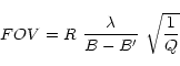$$FOV = R\ \frac{\lambda}{B-B^{\prime}}\ \sqrt{\frac{1}{Q}}$$ (3)

with $R(=\lambda/\Delta\lambda)$ the spectral resolution, B the length of the entrance baseline, $B^{\prime}$ the length of the exit baseline, and 1/Q the dynamic range. One can easily see that the contrast loss can be decreased by using small band filters or dispersion of the signal, enlarging the interferometric field-of-view.

For example, a measurement with the MIDI instrument on VLTI's telescopes UT1 and UT4 (130m baseline) at $10\,\mu$m in coaxial beam combination, with a dynamic range of 1/100 and a field-of-view with the size of an Airy disk requires a spectral resolution of $R\,=\,150$, smaller than the one which the instrument provides ( $R\,\geq{}\,200$).