Having understood the origin of the specific shape of the line-strength distribution function and its impact on the force-multiplier parameters in detail, we are now able to consider the question raised at the beginning of this paper, namely in how far the situation changes for different wind conditions. We will concentrate here on principal effects which are valid under fairly general circumstances. In particular, let us firstly consider the consequences if the overall metallicity is changed.
Due to its definition (6), the line-strength scales with metallicity (under the realistic assumption that the ionization balance is not severely modified) as
 |
(78) |
where z is the actual abundance ![]() relative to its solar value,
relative to its solar value,
![]() .
Thus, the major effect of changing the metallicity
is a shift of the according line-strength distribution functions (in the
.
Thus, the major effect of changing the metallicity
is a shift of the according line-strength distribution functions (in the
![]() representation) to the "left'' (for z < 1) or to the
"right'' (for z > 1).
representation) to the "left'' (for z < 1) or to the
"right'' (for z > 1).
Figure 26 verifies this behaviour for some exemplaric
atmospheric conditions (
![]() K and
K and ![]() K, respectively) and
three different metallicities, namely z=1 (solar), z=0.1 (roughly SMC)
and z=3 (typical for the Galactic center). The shift to lower/higher
line-strengths is clearly visible. Only for the largest line-strengths at
K, respectively) and
three different metallicities, namely z=1 (solar), z=0.1 (roughly SMC)
and z=3 (typical for the Galactic center). The shift to lower/higher
line-strengths is clearly visible. Only for the largest line-strengths at
![]() K the distributions seem to be unaffected by
metallicity, which is not surprising since the participating lines
are transitions from the hydrogen Lyman series (cf. Sect. 4.2.6).
K the distributions seem to be unaffected by
metallicity, which is not surprising since the participating lines
are transitions from the hydrogen Lyman series (cf. Sect. 4.2.6).
If we try to translate the shift in metallicity (affecting the independent
variable ![]() )
into the corresponding shift of the dependent variable
)
into the corresponding shift of the dependent variable
![]() ,
this relates to a modification of the vertical offset of the
distribution, i.e., of the normalization constant, or, in other words, of the
total number of contributing lines. In case of a perfect power-law then,
the normalization varies according to
,
this relates to a modification of the vertical offset of the
distribution, i.e., of the normalization constant, or, in other words, of the
total number of contributing lines. In case of a perfect power-law then,
the normalization varies according to
Since the force-multiplier parameter
![]() is proportional to
is proportional to ![]() (Eq. 12), it should scale according to
(Eq. 12), it should scale according to
With respect to ![]() and from its definition (37), obviously
and from its definition (37), obviously
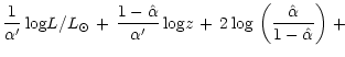
| (81) |
is predicted (cf. Gayley [1995]), (almost) independent from the specific shape of the line distribution.
|
|
z |
|
|
|
|
|
| 40000 | 3.0 | -0.98 | 0.68 | -0.98 | 0.69 | 5817 |
| 1.0 | -1.12 | 0.67 | -1.15 | 0.69 | 1941 | |
| 0.1 | -1.28 | 0.62 | -1.42 | 0.67 | 196 | |
| 10000 | 3.0 | -0.41 | 0.47 | -0.52 | 0.52 | 997 |
| 1.0 | -0.51 | 0.43 | -0.64 | 0.47 | 767 | |
| 0.1 | -0.87 | 0.36 | -0.96 | 0.40 | 663 |
In Table 3 we have calculated the f.m. parameters for the same
"models'' as in Fig. 26. The last column shows the validity
of the linear dependence
![]() for the hotter atmospheres, whereas
for the cooler ones
for the hotter atmospheres, whereas
for the cooler ones ![]() remains much more constant. If we remember that
remains much more constant. If we remember that
![]() is dominated by lines of maximum strength (Sect. 2.6 and Appendix C),
this behaviour results from the fact that the strongest driving lines in
this temperature domain are those from hydrogen and thus remain rather
unaffected by a change of global metallicity. Again, the conceptual
simplicity of the
is dominated by lines of maximum strength (Sect. 2.6 and Appendix C),
this behaviour results from the fact that the strongest driving lines in
this temperature domain are those from hydrogen and thus remain rather
unaffected by a change of global metallicity. Again, the conceptual
simplicity of the ![]() -approach is hampered by additional effects
becoming obvious only by means of detailed calculations.
-approach is hampered by additional effects
becoming obvious only by means of detailed calculations.
The other columns display the
![]() and
and
![]() values derived by
linear regressions to the calculated force-multipliers, both in the range of
values derived by
linear regressions to the calculated force-multipliers, both in the range of
![]() ("1'') as well as in the range of
("1'') as well as in the range of
![]() ("2'') with optical depth parameter
("2'') with optical depth parameter
![]() .
From the
differences, it is immediately clear that the assumption of a more or less
perfect power-law is only valid for the hotter atmosphere and low to
intermediate line-strengths, consistent with the run of
.
From the
differences, it is immediately clear that the assumption of a more or less
perfect power-law is only valid for the hotter atmosphere and low to
intermediate line-strengths, consistent with the run of
![]() shown in Fig. 27. Thus, the predicted scaling of
shown in Fig. 27. Thus, the predicted scaling of
![]() (Eq. 80) is only verified for case "2'' at 40000 K, whereas in
all other cases the reaction of
(Eq. 80) is only verified for case "2'' at 40000 K, whereas in
all other cases the reaction of
![]() is much weaker.
is much weaker.
One should note, however, that the primary influence of
![]() regards the
definition of the mass-loss rate. Thus,
regards the
definition of the mass-loss rate. Thus,
![]() is most important in the
subcritical region of the wind, where
is most important in the
subcritical region of the wind, where ![]() is low (and t is large), and
the contributing range in
is low (and t is large), and
the contributing range in ![]() is also small (typically 2 dex). Under
those conditions, however, a power-law distribution with
is also small (typically 2 dex). Under
those conditions, however, a power-law distribution with
![]() can be always justified (cf. Sect. 2.3.2), so that the effective
can be always justified (cf. Sect. 2.3.2), so that the effective
![]() -value controlling the mass-loss rate should actually
scale with (80), provided we compare winds of similar density. In
so far, the variations displayed in Table 3 are an artefact of the
much larger range of regression applied.
-value controlling the mass-loss rate should actually
scale with (80), provided we compare winds of similar density. In
so far, the variations displayed in Table 3 are an artefact of the
much larger range of regression applied.
 ''-effect for low metallicity and thin
winds
''-effect for low metallicity and thin
winds
Besides the obvious direct effect that the cumulative number of lines varies
in concert with z, we have to account for an additional complication: By
comparison of the various
![]() values derived by linear regression,
we find that also
values derived by linear regression,
we find that also
![]() is a function of metallicity, especially for
cooler temperatures. Regarding the difference between actual
(Fig. 27) and "power-law'' fitted values, the depth-dependent values of
is a function of metallicity, especially for
cooler temperatures. Regarding the difference between actual
(Fig. 27) and "power-law'' fitted values, the depth-dependent values of
![]() are typically smaller than the mean
for large
are typically smaller than the mean
for large ![]() ,
whereas they are larger or similar at low
,
whereas they are larger or similar at low ![]() -values. (Due
to the dominance of hydrogen lines with their
-values. (Due
to the dominance of hydrogen lines with their
![]() statistics, for
the cooler atmosphere we even encounter an - otherwise untypical - steep
increase of
statistics, for
the cooler atmosphere we even encounter an - otherwise untypical - steep
increase of
![]() towards maximum
towards maximum ![]() ).
).
The reason for the outlined behaviour is, again, the steep decline of
the line-strength distribution at its upper end, due to the excitation
effects discussed extensively in Sect. 4.2, and the horizontal shift of the
distribution as a function of metallicity. Thus, for lower z the steeper end
of the distribution becomes visible at lower values of ![]() ,
and
,
and
![]() can be roughly expressed as
can be roughly expressed as
neglecting certain subtleties arising from non-metallic lines.
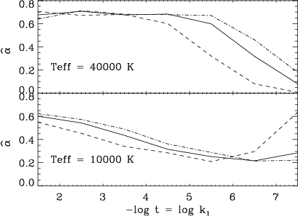 |
Figure 27:
As Fig. 26, however for
|
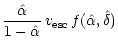
Whereas ![]() is an (almost) density independent quantity,
is an (almost) density independent quantity,
![]() scales with the inverse of the mean wind
density (times
scales with the inverse of the mean wind
density (times
![]() ). Thus, in addition to the metallicity shift
(argument of rhs in Eq. (82)), the range of
). Thus, in addition to the metallicity shift
(argument of rhs in Eq. (82)), the range of
![]() present
in the wind is also shifted compared to solar conditions. Since a reduced
metallicity yields a reduced wind density, this shift is towards higher
present
in the wind is also shifted compared to solar conditions. Since a reduced
metallicity yields a reduced wind density, this shift is towards higher
![]() ,
i.e., a low-metallicity wind plasma "doubles'' the effect of lowering
,
i.e., a low-metallicity wind plasma "doubles'' the effect of lowering
![]() .
In contrast, enhanced metallicities have almost no effect on
.
In contrast, enhanced metallicities have almost no effect on
![]() ,
since the corresponding shift is towards lower
,
since the corresponding shift is towards lower ![]() ,
where the
line-strength distribution function has a more constant slope.
,
where the
line-strength distribution function has a more constant slope.
Of course, the described process is also present if the wind-density is low for
other reasons, e.g. because the luminosity is low. Compared to supergiant
winds then, the ![]() range to be considered is shifted towards higher
values, and
range to be considered is shifted towards higher
values, and
![]() is accordingly lower.
is accordingly lower.
In conclusion, thin and fast winds as well as low metallicity winds tend to
have lower
![]() -values than high density or high metallicity winds,
both on the average as well as locally. Once more, the reason for this
effect is the curvature of the line-strength distribution function,
especially at highest line-strengths, which is also the answer to the
problem raised at the end of Sect. 2.5 concerning the origin of the lower
-values than high density or high metallicity winds,
both on the average as well as locally. Once more, the reason for this
effect is the curvature of the line-strength distribution function,
especially at highest line-strengths, which is also the answer to the
problem raised at the end of Sect. 2.5 concerning the origin of the lower
![]() -values calculated in a low metallicity environment. If, on the
other hand, a perfect power-law were present,
-values calculated in a low metallicity environment. If, on the
other hand, a perfect power-law were present,
![]() ,
independent on wind density and metallicity.
,
independent on wind density and metallicity.
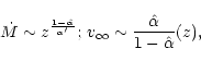
As a consequence of the variations of
![]() as a function of
as a function of ![]() ,
,
![]() varies throughout the wind, since
varies throughout the wind, since ![]() changes by typically three dex from inside to outside
changes by typically three dex from inside to outside![]() .
Hence, any exact hydrodynamic solution requires depth dependent
force-multipliers (cf. Kudritzki et al. [1998])
.
Hence, any exact hydrodynamic solution requires depth dependent
force-multipliers (cf. Kudritzki et al. [1998])
At this point of reasoning, we like to reiterate our findings in a somewhat
different context. From our experience, the behaviour of the line-force in a
low-density environment is frequently misinterpreted. E.g., after having
calculated the according f.m. parameters - with the result of
![]() in the outermost wind part -, there seems to be a common concern
whether this is not only an artefact of an incomplete line-list at lower
gf-values. Actually, however, almost the opposite effect is present! If,
e.g. in B-dwarf winds, the density becomes so low that
in the outermost wind part -, there seems to be a common concern
whether this is not only an artefact of an incomplete line-list at lower
gf-values. Actually, however, almost the opposite effect is present! If,
e.g. in B-dwarf winds, the density becomes so low that
![]() (corresponding to
(corresponding to
![]() ), all lines contribute to the
line-acceleration at their optically thin limit,
), all lines contribute to the
line-acceleration at their optically thin limit,
![]() .
Thus, the strongest (however optically thin) lines have the largest
influence and the numerical value of the total force does not depend on any
incompleteness of the line list at low gf-values. The fact that
.
Thus, the strongest (however optically thin) lines have the largest
influence and the numerical value of the total force does not depend on any
incompleteness of the line list at low gf-values. The fact that ![]() tends to zero in this case is, as explained already in Sect. 2.3, given by
the independence of the line-force on any variation of t (or
tends to zero in this case is, as explained already in Sect. 2.3, given by
the independence of the line-force on any variation of t (or ![]() ).
).
With respect to the horizontal shift "to the left'' in a low-metallicity
environment, this independence on ![]() can start even earlier, i.e., the
line-force becomes saturated (
can start even earlier, i.e., the
line-force becomes saturated (
![]() )
at lower values of
)
at lower values of ![]() .
Even in cases of a higher metallicity (where the effects of an incomplete
line-list may become obvious at least in principle), the actual range of
contributing
.
Even in cases of a higher metallicity (where the effects of an incomplete
line-list may become obvious at least in principle), the actual range of
contributing ![]() values is normally much too small that this might become
a real problem.
values is normally much too small that this might become
a real problem.
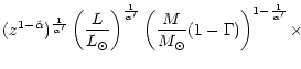
Including now the aforementioned finite disk correction factor and
accounting for ionization effects
![]() ,
we
can summarize the resulting scaling relations for
,
we
can summarize the resulting scaling relations for ![]() and
and
![]() as
function of metallicity, which arise if a metal dependent line-force
is used to solve the hydrodynamic equations (for actual solution methods,
cf. PPK and Kudritzki et al. [1989]) and the f.m. parameters were
constant throughout the wind:
as
function of metallicity, which arise if a metal dependent line-force
is used to solve the hydrodynamic equations (for actual solution methods,
cf. PPK and Kudritzki et al. [1989]) and the f.m. parameters were
constant throughout the wind:
 |
|||
| (83) | |||
| = |  |
(84) | |
| = | (85) | ||
| g | 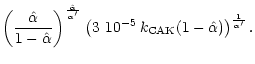 |
(86) |
M is the stellar mass and
![]() the escape velocity, corrected for
the Eddington factor
the escape velocity, corrected for
the Eddington factor ![]() .
.
![]() is a decreasing
function of
is a decreasing
function of
![]() ,
and has a value of roughly 2.2 if
,
and has a value of roughly 2.2 if
![]() is small (cf. Kudritzki et al. [1989]). The function g finally
accounts for the (moderate) dependence on terms of order
is small (cf. Kudritzki et al. [1989]). The function g finally
accounts for the (moderate) dependence on terms of order
![]() ,
on
the proportionality to
,
on
the proportionality to
![]() ,
and, most important (and frequently
forgotten), on the scaling factor
,
and, most important (and frequently
forgotten), on the scaling factor
![]() , since the mass-loss
rate actually depends on the Eddington factor
, since the mass-loss
rate actually depends on the Eddington factor
![]() and not
on
and not
on
![]() itself. Note, that the variation of g has to be
considered in any comparison where
itself. Note, that the variation of g has to be
considered in any comparison where
![]() is different (e.g., A-star vs. O-star winds, see below).
is different (e.g., A-star vs. O-star winds, see below).
In case of depth dependent parameters, ![]() relates to the conditions at
the critical point (
relates to the conditions at
the critical point (
![]() for not too thin winds), where
for not too thin winds), where
![]() and
and
![]() do not vary heavily. The terminal velocity,
however, is dependent on some average value of
do not vary heavily. The terminal velocity,
however, is dependent on some average value of
![]() between the location of the critical point and large values of
between the location of the critical point and large values of ![]() ,
and
will be typically smaller compared to using the
,
and
will be typically smaller compared to using the
![]() values present
at the critical point, because of the reasons outlined above.
values present
at the critical point, because of the reasons outlined above.
In any case, to first order we find the metallicity effect as
 |
(87) |
which, in case of O-star winds (small
![]() )
yields the often
quoted scaling relation for the mass-loss rate
)
yields the often
quoted scaling relation for the mass-loss rate
![]() since
since
![]() .
.
Due to the metallicity dependent factor
![]() ,
one
can expect lower terminal velocities in a metallicity-deficient environment.
This is just what has been found by comparing O-star terminal velocities in
the Galaxy and the Clouds, cf. Fig. 28. For a detailed discussion,
we refer the reader to the papers by Garmany & Conti ([1984]),
Kudritzki et al. ([1987]), Haser et al. ([1993]) and
Walborn et al. ([1995]).
,
one
can expect lower terminal velocities in a metallicity-deficient environment.
This is just what has been found by comparing O-star terminal velocities in
the Galaxy and the Clouds, cf. Fig. 28. For a detailed discussion,
we refer the reader to the papers by Garmany & Conti ([1984]),
Kudritzki et al. ([1987]), Haser et al. ([1993]) and
Walborn et al. ([1995]).
| |
Figure 28: Terminal velocities of O-type stars in the Galaxy and the Magellanic clouds. Data from Haser ([1995]) and Puls et al. ([1996]) |
| |
Figure 29: Wind momentum (in cgs units) and luminosity of galactic and SMC supergiants and two A-supergiants in M 33. Open square: M 33 A-supergiant with galactic metallicity. Cross: Extremely metal poor A-supergiant in the outskirts of M 33. (From McCarthy et al. [1995]) |
Finally and with respect to the wind-momentum luminosity relation (Kudritzki et al. [1995]; Puls et al. [1996]), our findings imply (leading terms only)
where, of course, in case of
![]() an additional
correction for mass effects might be necessary.
an additional
correction for mass effects might be necessary.
From the presently available data, it is clear that at least in the SMC a
different offset is visible (due to the second term in the above equation,
resulting from the "direct'' effect (cf. Fig. 29, and also Puls
et al. [1996]; Kudritzki [1997]). Whether there is actually
a different slope (as a consequence of a reduced ![]() ), is not certain
due to the small number statistics for SMC O-stars. To clarify the
situation, more objects have to be analyzed. This work is well under way in
our group.
), is not certain
due to the small number statistics for SMC O-stars. To clarify the
situation, more objects have to be analyzed. This work is well under way in
our group.
Contrasted to the above uncertainty concerning the reduction of
![]() in a metal poor environment, the observational status quo with respect to
the difference of A-star vs. O-star winds is much more promising. From the
latest results by Kudritzki et al. ([1999]), the WLR for Galactic
A-Supergiants (in a temperature range
in a metal poor environment, the observational status quo with respect to
the difference of A-star vs. O-star winds is much more promising. From the
latest results by Kudritzki et al. ([1999]), the WLR for Galactic
A-Supergiants (in a temperature range
![]() K) reads
K) reads
![]() ,
to be compared with the
relation valid for Galactic O-Supergiants (from Puls et al.
[1996]),
,
to be compared with the
relation valid for Galactic O-Supergiants (from Puls et al.
[1996]),
![]() .
.
Note at first that the observed slope (interpreted as
![]() )
lies exactly in the range to be expected for
A-type winds, cf. Tables
2 and 3. Second, from the difference in the
offset compared to O-stars (
)
lies exactly in the range to be expected for
A-type winds, cf. Tables
2 and 3. Second, from the difference in the
offset compared to O-stars (
![]() ), we can calculate the
average value of the parameter
), we can calculate the
average value of the parameter
![]() (A-SG) using Eq. (88), the values
found for
(A-SG) using Eq. (88), the values
found for ![]() from the WLRs and the appropriate values for
from the WLRs and the appropriate values for
![]() and
and
![]() K) from Table 3. In result, we find
K) from Table 3. In result, we find
![]() (A-SG) = -0.84. This number is reasonable when compared to
our theoretical prediction
(A-SG) = -0.84. This number is reasonable when compared to
our theoretical prediction
![]() K) = -0.51
(Table 3) at
K) = -0.51
(Table 3) at
![]() ,
accouting for the fact that
A-Supergiants have lower densities at the critical point (smaller
,
accouting for the fact that
A-Supergiants have lower densities at the critical point (smaller ![]() and larger radii) than their O-type counterparts. In so far, the difference
found is a consequence of the
and larger radii) than their O-type counterparts. In so far, the difference
found is a consequence of the ![]() -term, which is implicitely included in the value of
-term, which is implicitely included in the value of
![]() derived in our comparison.
derived in our comparison.
Thus, we conclude that our theoretical predictions concerning the run
of
![]() (and
(and
![]() )
with respect to temperature are correct, and,
additionally, in Sect. 4 we have explained the reason for this behaviour.
)
with respect to temperature are correct, and,
additionally, in Sect. 4 we have explained the reason for this behaviour.
Copyright The European Southern Observatory (ESO)