3 Line-strength distribution functions for stellar wind conditions and the validity of Gayley's Ansatz

In the previous sections, we have shown that under quite general conditions the summation of individual line accelerations leads to the CAK law $g_{\rm rad}^{\rm tot} \propto k_{\rm 1}^{\hat \alpha}$, where $\hat \alpha$ follows the local slope of the line-strength distribution function as long as this is not too steep.

Although the limiting values of $\hat \alpha=0 \ldots 1$ are obvious by definition, nothing has been said so far concerning its specific value. The importance of this quantity has been pointed out in the introduction and shall be stressed once more: To understand the basic wind physics and to be able to obtain quantitative predictions (as, e.g., via Eqs. (41) or (42)), a thorough discussion of the line-strength distribution and its dependence on different quantities such as wind density, metallicity etc. is inevitable. Before doing this in Sects. 4 and 5, we will describe our method of calculating those distribution functions, derive force-multiplier parameters and comment on the presumed equality of $\bar Q$ and $Q_{\rm o}$.

3.1 Data and basic approximations

3.1.1 Atomic data

The data base upon which this work is based has been compiled over the last 15 years by A. Pauldrach in collaboration with one of us (M.L.). The wavelengths, gf-values, photoionization cross sections and collision strengths for a total of 149 ionization stages and 2.5 million lines are stored (for the highest ionization stage of the elements see Table 1). The considered elements are hydrogen to zinc except lithium, beryllium, boron and scandium which are too rare to play a role in radiative line driving. The origin of the data has recently been described by Pauldrach et al. ([1998]). Note, that each model ion considered in NLTE consists of carefully chosen levels (typically of order 50), which are sufficient to define the most important occupation numbers required for calculating the line-force, as long as the line list is complete. For light ions, the highest considered level lies close to the ionization edge, whereas for the heavy elements the cutoff was chosen in such a way to include all meta-stable levels and levels above which are significantly populated.

Of course, the completeness of the data in terms of their potential contribution to radiative driving is a critical issue. Apart from the high frequency cutoff given by the highest represented ionization stages (thereby effectively limiting the usefulness of the line database for computing radiation pressure to stars with $T_{\rm eff}< 100\,000\, {\rm K}$) there is the question of how many weak lines have to be represented to regard the list as essentially complete. Comparisons have been made (see Springmann [1997]) with the line opacity data from the Opacity Project (Seaton [1995]) and the Kurucz data (Kurucz [1995]). After gaps in line opacity due to missing data in the UV spectral range in our database were closed, all three data collections now agree in their spectral line opacity distribution.

Since the Kurucz data base is the most complete now in existence we conclude that we are as complete as presently possible. Furthermore, tests made by omitting the weakest lines have shown that their contribution is negligible so that further enhancements of line opacity redward of 229 Å are not expected.

 

 

Table 1: The highest ionization stage considered in our database. Carbon to Calcium: "light ions''; Titanium to Zinc: "iron group elements''

Elem.	max. ion.	Elem.	max. ion.	Elem.	m. ion.
H	I	He	II
C	V	N	VI	O	VI
F	VI	Ne	VI	Na	VI
Mg	VI	Al	VI	Si	VI
P	VI	S	VII	Cl	VI
Ar	VIII	K	VI	Ca	VI
Ti	V	V	V	Cr	VI
Mn	VI	Fe	VIII	Co	VII
Ni	VIII	Cu	VI	Zn	III

3.1.2 Approximate non-LTE occupation numbers

To determine the line-strengths for atomic transitions under stellar wind conditions one has to know the occupation numbers of the corresponding levels (see Eq. 5). To keep matters simple we have employed the following assumptions (for a thorough discussion, cf. Springmann [1997]):

Ionization equilibrium.

The ionizing radiation field is approximated by $J_\nu = W I_\nu(T_{\rm rad})$, where the intensity $I_\nu$ is taken either as Planck or from a Kurucz model atmosphere (Kurucz [1995]). Since the atmospheric conditions are specified at one point only, the dilution factor is a numerical factor of order 1 ... 0.001. With the electron temperature taken as a constant fraction of the effective temperature (typically 0.8) and the radiation temperature as either the effective one (Planck case) or lower (Kurucz fluxes), the ionization equilibrium reads

 

$$\frac{n_{1,j+1} n_{\rm e}}{n_{1,j}} W \sqrt{\frac{T_{\rm e}}{T_{\rm rad}}} \left(\frac{n_{1,j+1} n_{\rm e}}{n_{1,j}}\right)^*_{T_{\rm rad}}$$ =

$$\times \left\{\zeta + \eta + W (1-\eta - \zeta)\right\}.$$ (43)

The asterisk denotes thermodynamic equilibrium values and $\zeta$ and $\eta$are the fraction of recombination processes leading directly to the ground and meta-stable levels, respectively. The underlying assumptions leading to this equation (which goes back to unpublished notes by Leon Lucy) are: The ionization balance is dominated by radiative processes and given by the equilibrium of photoionization processes from all levels and recombination processes to all levels. Line transitions are considered as optically thin (i.e., the action of line transitions on the level populations is neglected; see below). The frequency dependence of the photoionization cross section is taken as a quadratic decline from the edge value; tests have shown that for a wide variety of parameterizations the error incurred does not exceed 10%. Equation (43) has a smooth transition to the LTE-Regime for $W \to 1$. A similar equation (but without the $\eta$-terms) has been employed by Schmutz ([1991]) and Schaerer & Schmutz ([1994]).

Level occupation numbers.

Having determined the ionization equilibrium, the distribution of the ions on the level states follows the Abbott & Lucy ([1985]) prescription: meta-stable states have equilibrium populations relative to the ground state ( $n_m/n_1 = (n_m/n_1)^*_{T_{\rm rad}}$), other levels have a diluted population ( $n_i/n_l = W (n_i/n_l)^*_{T_{\rm rad}}$) relative to either the ground state or a meta-stable state, depending on which lower state corresponds to the strongest downward transition. Excited levels which do not have a direct downward transition to either the ground or a meta-stable level are neglected. The transitions which have one of the three classes of levels as lower levels (i.e., resonance transitions, quasi-resonance transitions starting from a meta-stable level and 1st order subordinate transitions) contribute most of the line opacity. In this way it is possible to specify the level occupations without actually solving the rate equations.

This prescription for the the level occupations can be justified by considering a 3-level atom neglecting collisions and line optical thickness (in large distances from the star the mean intensity in optically thick lines decreases faster than in optically thin lines). This last assumption is hardly important, however, since it mainly affects the upper levels of a transition which have a negligible influence on the line optical thickness. Meta-stable levels are not affected since they are populated from higher levels (direct downward transitions are forbidden by definition). Collisions are important for high densities but here our prescription ensures a smooth transition to LTE both for the ionization and excitation structure. These assumptions are of greater importance when computing complete wind models with a radial stratification in all variables whereas for our present purposes they do not matter since we do not consider a specific model.

The end result of all approximations compares favourably with the much more detailed non-LTE-calculations by Pauldrach et al. ([1994]) with respect to both the ionization balance and the emergent flux (see the example for the O4If star $\zeta$-Pup in Springmann & Puls [1998]).

3.2 Line-strength distribution functions and force-multiplier parameters for some examples

Having calculated the occupation numbers for all involved levels, the line-strengths of all transitions in our data base can be found by means of Eq. (6) and the distribution functions derived. In the following sections, we will display either the differential form, where we bin (if not stated explicitly else) the number of lines $\Delta N$ per 0.5 dex in line-strength and 5 kiloKayser (kK, 1 Kayser = 1 cm^-1) in frequency, or we show the cumulative line-strength distribution, i.e, the number of lines $N(k_{\rm L})$ with strengths larger than $k_{\rm L}$. Flux (times frequency) weighted functions differ by the additional weight $\nu_{\rm i}F_{\nu}/F$, where F is the integrated flux, assumed to be Planck in this section (using appropriate Kurucz fluxes will change only some quantitative, however not qualitative conclusions, cf. Sect. 4.2.8). The local slope of this distribution, in the log-log representation, then corresponds to $\alpha -1$.

Force-multipliers are calculated by explicitly summing up the individual components (Eq. 17) as function of given depth parameters $t = k_{\rm 1}^{-1}$ and normalizing to the Thomson acceleration. If we are interested also in $\hat \delta$, the whole procedure is repeated for different values of $n_{\rm e}/W$ controlling the ionization/excitation balance. $\hat \alpha$ and $\hat \delta$ are then found from local logarithmic derivatives with respect to t and $n_{\rm e11}/W$, where $n_{\rm e11}$ is the electron density in units of $10^{11}~{\rm cm}^{-3}$.

Typical examples for the total variation of $\hat \alpha$ and $\hat \delta$ are given in Sect. 4, here we will constrain ourselves to the case of a fixed value of $n_{\rm e11}/W = 10, W = 0.33$ and various effective temperatures in the range between 50000...10000 K.

 

 

Table 2: Various force-multiplier parameters as function of $T_{\rm eff}$, for $n_{\rm e11}/W = 10$ and W = 0.33 (see text)

$T_{\rm eff}$	${\rm log}\, k_{\rm CAK}$	$\hat \alpha$	$\bar Q$	$Q_{\rm o}$	${\rm log}\, k_{\rm CAK}$
					$(Q_{\rm o}=\bar Q)$
50000	-1.11	0.66	1939	2260	-1.06
40000	-1.13	0.67	1954	1778	-1.15
30000	-1.08	0.64	2498	3630	-0.97
20000	-1.02	0.58	1597	5171	-0.72
10000	-0.54	0.44	915	14505	-0.01

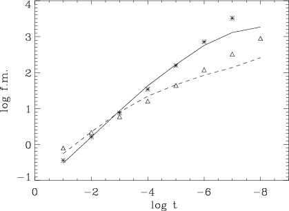Figure 2: Log force-multiplier as function of ${\rm log}\,t = - {\rm log}\, k_{\rm 1}$, for the models with $T_{\rm eff}$ = 50000 K (fully drawn) and 10000 K (dashed). For parameters, see Table 2. Asterisks and triangles gives linear regression for $\hat \alpha$ in the range ${\rm log}\,t = -1 \ldots -6$

Figure 3: (Planck-)Flux weighted cumulative line-strength distribution function, for the models with $T_{\rm eff}$ = 50000 K (fully drawn) and 10000 K (dashed). For parameters, see Table 2. Vertical lines give line-strengths corresponding to $Q_{\rm o}$ (calculated from $\bar Q, k_{\rm CAK}, \alpha$, cf. Eq. (38)) for the appropriate model. Note, that the cutoff of the distribution functions lies exactly at the calculated value!

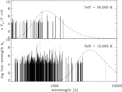Figure 4: Frequential distribution of the strongest lines ( ${\rm log}\, k_{\rm L}\ge 4$) for the models of Fig. 3, in the range 200 to 10000 Å. Lines from hydrogen and helium are indicated by dots. Overplotted is the frequential weight factor $\nu F_{\nu }/F$, magnified by a factor 10

At first, let us concentrate on the force-multipliers. Table 2 gives the values of $k_{\rm CAK}$ and $\hat \alpha$ as function of temperature, which in this case were calculated by a linear regression ${\rm log}$ f.m. versus ${\rm log}\, t$ for the range ${\rm log}\,t = -1 \ldots -6$. Figure 2 shows the corresponding function for the borders of our temperature range. The behaviour is rather monotonic: $k_{\rm CAK}$ increases with decreasing temperature, indicating an increasing potential of flux-blocking, and $\hat \alpha$ decreases from the canonical value 2/3 to 0.44 at the lowest temperature. Note, that the actual force-multiplier shows an almost exactly constant slope in the hot wind case, whereas for the cool temperature a curvature is present.

3.3 Validity of Gayley's Ansatz

For the models displayed, we have calculated $\bar Q$ from Eq. (37), and, by comparing with the corresponding value of $k_{\rm CAK}$, derived the $Q_{\rm o}$value implied by (38). At first note that $\bar Q$ lies exactly in the range given by Gayley, and that especially at the hotter temperatures the favourized value of 2000 is exactly met. Second, $\bar Q$ decreases to lower temperatures, again in concert with the findings by Gayley. However, it is also obvious, that the (power-law) "equality'' $Q_{\rm o} = \bar Q$(Gayley's Ansatz!) is only met by the hotter models, whereas for the cooler ones a mismatch beyond a factor of ten is present.

The last panel in Table 2 gives the resulting $k_{\rm CAK}$-value if $Q_{\rm o} = \bar Q$ actually would have been set. Clearly, this assumption leads to much too large $k_{\rm CAK}$'s, or, in other words, the estimated mass-loss rates would be much too high!

Let us firstly check whether the $Q_{\rm o}$-values derived from our line-force parameterization (38) and $\bar Q$ have anything to do with reality. For this reason, Fig. 3 displays the corresponding line-strength distribution functions, flux-weighted and cumulative. At first note the strong correspondence with the force-multiplier plot from above. For the hot wind, the slope is almost constant, which is the final reason that also the f.m. plot displays this behaviour, as explained in Sect. 2. In contrast, for the cooler temperature the distribution is curved, and the transition point between a rather steep (low $\alpha$) and a flatter slope is located at the same line-strength as in the f.m. plot, namely at ${\rm log}\,k_{\rm L}= 4$corresponding to ${\rm log}\, t = -4$.

We have indicated the calculated values of $Q_{\rm o}$ (translated to $k_{\rm L}$) by vertical lines. Obviously, they have the correct order of magnitude, which is also true for the other three models which are not displayed. This result tells us that at least globally the assumption of a power-law distribution (required to validate Eq. (38)) seems to be justified, although the precise numbers (which are important for quantitative predictions since ${\dot M}/L \propto Q_{\rm o}^{-1}$ if $Q_{\rm o} \ne \bar Q$) depend on the curvature of the distribution, of course.

Since we have displayed the flux (times frequency) weighted distribution function required to calculate line-forces, the value of $\left\langle N(k_{\rm max}) \right\rangle$ gives some information about the frequential position of the strongest line(s). Whereas for the hotter atmosphere this number is close to unity (i.e., the strongest lines are close to flux maximum), the significantly lower value for the cooler atmosphere immediately points to the fact that here the strongest lines are disconnected from the maximum.

This obviously increasing mismatch between the position of the strongest lines and the flux-maximum is, besides the discussed influence of curvature terms, the primary reason for the "observed'' difference between $\bar Q$and $Q_{\rm o}$ (for details, see Appendix C). In Fig. 4 we have indicated the frequential line distribution for all lines with ${\rm log}\, k_{\rm L}> 4$, overplotted by the according flux weighting factor $L_{\nu_{\rm i}} \nu_{\rm i}/L$(magnified by a factor of ten for convenience). In accordance with the previous figure, the lines for the hotter model are almost uniformly distributed over the total contributing frequential regime. The cooler one, however, has its maximum density of strong lines in the Wien-regime of the radiation field. This behaviour bases on the fact that (for all temperatures and "normal'' composition) the strongest lines (excluding H/He) are the resonance lines of the CNO-group (Sect. 4.2.6) which are located, independently of ionization, in the UV. (E.g., the positions of the (second strongest) C II and O VI resonance lines at $\sim 1030$ Å are almost identical.) In consequence, the average weight factor of the strongest lines which dominate $\bar Q$ is decreasing for decreasing temperature and leads, as discussed in Appendix C, to an increasing ratio of $Q_{\rm o}/\bar Q$.

In conclusion, our comparison has shown that the principle formalism provided by Gayley is valid to the same degree of precision than the older CAK parameterization. At least for the cooler stars, however, one has to account for the presence of an average $\bar Q$ (much) smaller than the maximum line-strength $Q_{\rm o}$. In so far, the problem of a rather unpredictable behaviour of $k_{\rm CAK}$ (if one has no tool to calculate it) is replaced by the simultaneously unknown ratio of $\bar Q/Q_{\rm o}$. Only in cases when the frequential distribution is uniform and the line-strength distribution has a constant slope, $Q_{\rm o}$ = $\bar Q$ can be set. Thus, only simple cases (hot Supergiant winds) can be treated by the simple version of the formalism, whereas in all other cases (thin, metal-poor or cooler winds) at least one of the above problems prevents a blind application.