7 The fitting functions

The main aim of this work is to derive empirical fitting functions for the D₄₀₀₀ in terms of the stellar atmospheric parameters: effective temperature, metallicity and surface gravity. After some experimentation, we decided to use $\theta\equiv 5040/T_{\rm eff}$ as the temperature indicator, being [Fe/H] and $\log g$ the parameters for the metallicity and gravity. Following the previous works of G93 and W94, the fitting functions are expressed as polynomials in the atmospheric parameters, using two different functional forms:

 

$${ D}_{4000}(\theta,{\rm [Fe/H]},\log g) = p(\theta,{\rm [Fe/H]},\log g)$$ (11)

and  

$${ D}_{4000}(\theta,{\rm [Fe/H]},\log g) = {\rm const.} + {\rm e}^{p(\theta,{\rm [Fe/H]},\log g)} ,$$ (12)

where p is a polynomial with terms up to the third order, including all possible cross-terms among the parameters:

 

$$p(\theta,{\rm [Fe/H]},\log g) = \sum_{k=0}^{19} c_k\ \theta^i\ {\rm [Fe/H]}^j\ (\log g)^l,$$ (13)

with $0\leq i+j+l\leq3$.

  

Figure 6: Details of the fitting functions in the mid-temperature range for a) giant ($\log g<3.5$) and b) dwarf ($\log g\gt 3$) stars. See caption to Fig 5. Error bars for the D4000 measurements are also shown

  

Figure 7: Residuals of the derived fitting functions (observed minus predicted) against the three input stellar parameters. Symbol types are the same as in Fig. 3. The length of the error bar is twice the unbiased residual standard deviation

The polynomial coefficients were determined from a least squares fit where all the stars were weighted according to the D₄₀₀₀ observational errors listed in Table 1. Note that this is an improvement over the procedure employed by G93 and W94 for the Lick indices.

Obviously, not all possible terms are necessary. The strategy followed to determine the final fitting function is the successive inclusion of terms, starting with the lower powers. At each step, the term which yielded a lower new residual variance was tested. The significance of this new term, as well as those of all the previously included coefficients, was computed using a t-test (i.e. from the error in the coefficient, we tested whether it was significantly different from zero). Note that this is equivalent to performing a F-test to check whether the unbiased residual variance is significantly reduced with the inclusion of the additional term. Following this procedure, and using typically a significant level of $\alpha=0.10$, only statistically significant terms were retained. The problem is well constrained and, usually, after the inclusion of a few terms, a final residual variance is asymptotically reached and the higher order terms are not statistically significant. Throughout this fitting procedure we also kept an eye on the residuals to assure that no systematic behaviour for any group of stars (specially stars from any given cluster or metallicity range) was apparent.

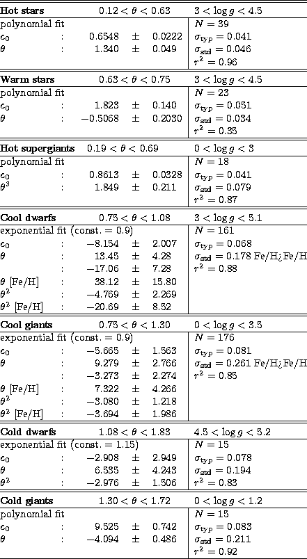
After a set of trial fits, it was clear that temperature is the main parameter governing the break. Unfortunately, the behaviour of the D₄₀₀₀ could not be reproduced by a unique polynomial function in the whole temperature range spanned by the library, forcing us to divide the temperature interval into several regimes. The derived composite fitting function is shown in Fig. 5. In Table 3 we list the corresponding coefficients and errors, together with the typical error of the N stars used in each interval ($\sigma_{\rm typ}^2=N/\sum_{i=1}^n \sigma_i^{-2}$), the unbiased residual variance around the fit ($\sigma_{\rm std}^2$) and the determination coefficient (r²).

  

Table 3: Parameters of the empirical fitting functions in each temperature and gravity range

In the high temperature regime ($\theta\leq0.75$, $T_{\rm eff}\geq\allowbreak 6700$ K) a dichotomic behaviour for dwarfs and giants on one side, and supergiants on the other, is clearly apparent. Therefore we derived different fitting functions for each gravity range. For the first group the amplitude of the break is quite constant and only the linear term in $\theta$ is statistically significant (note that we subdivide this range in two intervals to achieve a better fit). The independence on metallicity is naturally expected (see Sect. 2) but note that an important fraction of the stars in this range either lack of a [Fe/H] estimation or are restricted to the solar value.

The behaviour of the cool stars ($0.75\leq\theta\leq1.3$, $3900\ {\rm K}\leq T_{\rm eff}\leq 6700$ K) is more complex and [Fe/H] terms are clearly needed. On the other hand, no gravity term is significant. However, whilst for the giant stars D₄₀₀₀ increases with $\theta$ all the way up to $\theta\approx1.3$, for higher gravities it reaches a maximum at $\theta\approx1.1$ and then levels off. Furthermore, separate fits for dwarfs and giants in this $T_{\rm eff}$ range (with a gravity cutoff around 3-3.5) yield residual variances that are significantly smaller than the variance from a single fit. Hence, we have derived different fitting functions for dwarfs and giants. This dichotomic behaviour of the break is not surprising since its strength is quite dependent on the depth of the CN bands (Fig. 1) which also shows a similar behaviour (G93) due to the onset of the dredge-up processes at the bottom of the giant branch. In Fig. 6 we show in detail the fitting functions derived for each gravity group in this temperature range.

Concerning the cold stars ($\theta\geq1.3$, $T_{\rm eff}\leq3900$ K), the difference between giants and dwarfs is quite evident and two fitting functions have been derived (see also Sect. 2). Again, the metallicity terms are not significant, although this may be, at least in part, due to the paucity of input metallicities in this range. It must be noted that the different fitting functions have been constructed with the constrain of allowing for a smooth transition in the predicted D₄₀₀₀ indices among the different $T_{\rm eff}$ and gravity ranges.

In Fig. 7 we plot the residuals from the fits as a function of effective temperature, metallicity and gravity. Note that no trends are apparent with any of these parameters. We have also checked for systematic residuals within any of the star clusters. Except for an unexplained negative offset for the Coma stars ($\Delta{ D}_{4000}=0.09$, not due to an error in the adopted metallicity), no systematic offsets have been found. For the 420 stars used in the fit, we derive an unbiased residual standard deviation $\sigma_{\rm std}=0.160$. This must be compared with the typical error in the D₄₀₀₀, $\sigma_{\rm typ}=0.064$. Therefore, the residuals are, in the mean, a 2.5 factor larger than what should be expected solely from measurement errors. Since we are quite confident that these latter errors are realistic (see Sect. 5), and although some scatter may arise from the fact than the fitting functions are not able to reproduce completely the complex behaviour of the D₄₀₀₀, most of the extra scatter must arise form uncertainties in the input atmospheric parameters. For example, the residual D₄₀₀₀ scatter of 0.248 for the cool giants (at $\theta = 1.0$ and ${\rm [Fe/H]} = 0.0$) can be fully explained by the combined effect of a 166 K uncertainty in $T_{\rm eff}$ and a 0.29 dex error in [Fe/H], both consistent with the typical errors found by [53, Soubiran et al. (1998)] when comparing atmospheric parameters from the literature. Another quantitative measurement of the quality of the present fitting functions is the determination coefficient for the whole sample r²=0.96. This indicates that a 96% of the original variation of the break in the sample is explained by the derived fitting functions.

Since the goal of this work is to predict reliable D₄₀₀₀ indices for any given combination of input atmospheric parameters, we have investigated, using the covariance matrices of the fits, the random errors in such predictions. These errors are given in Table 4 for some representative sets of input parameters. Note that, as it should be expected, the uncertainties are smaller for near-solar metallicities. Interestingly, although the library does not include a high number of 0-B stars, the predicted indices at the hot end of the star sample are rather reliable.

  

Table 4: Uncertainties in the predicted D₄₀₀₀ values for some indicative sets of stellar parameters. For the cool stars ($T_{\rm eff}\leq6000~ {\rm K}$) the term giants refers also to supergiant stars