5 Random errors and systematic effects

  Since the aim of this paper is to derive an analytical representation of the behaviour of the D₄₀₀₀ as a function of effective temperature, metallicity and surface gravity, the sources of error are two-fold. In one hand, an important error source are the uncertainties in the adopted atmospheric stellar parameters. Detailed discussions of the sources of the stellar parameters and their associated errors are given in the original papers G93 and W94. In this work we assume that these errors are random and, thus, their effect in the fitting procedure is minimized through the use of a library containing a large number of stars. The other type of errors are those associated to D₄₀₀₀ measurements, which are the subject of this section. Undoubtly, an accurate knowledge of the errors is essential to guarantee the validity of the final product of this work, i.e., the fitting functions of the break.

Since, apart from the cluster members, most of the stars of the Lick/IDS library are bright, and considering the low signal-to-noise ratio required to measure the D₄₀₀₀ with acceptable accuracy, systematic errors are the main source of uncertainty.

5.1 Random errors

(i) Photon statistics and read-out noise. With the aim of tracing the propagation of photon statistics and read-out noise, we followed a parallel reduction of data and error frames. For a detailed description on the estimation of random errors in the measurement of line-strength indices we refer the interested reader to [14, Cardiel et al. (1998b)]. Starting with the analysis of the photon statistics and read-out noise, the reduction package REDucmE is able to generate error frames from the beginning of the reduction procedure, and properly propagates the errors throughout the reduction process. In this way, important reduction steps such as flatfielding, geometrical distortion corrections, wavelength calibration and sky subtraction, are taken into account. At the end of the reduction process, each data spectrum $S(\lambda_i)$ has its associated error spectrum $\sigma(\lambda_i)$, which can be employed to derive accurate index errors. The errors in the break are computed by [14, (Cardiel et al. 1998b)]  

$$\Delta^2[{ D}_{4000}]_{\rm photon} = \frac{ {\cal F}_r \sig... ...\cal F}_b}+ {\cal F}_b \sigma^2_{{\cal F}_r} }{ {\cal F}_b^4 },$$ (4)

with  

$${\cal F}_p \equiv \sum_{i=1}^{N_p} [\lambda_i^2 S(\lambda_i)],$$ (5)

and  

$$\sigma^2_{{\cal F}_p} = \Theta^2 \sum_{i=1}^{N_p} [\lambda_i^4 \sigma^2(\lambda_i)],$$ (6)

where the subscripts b and r correspond, respectively, to the blue and red bandpasses of the break (p refers indistinctly to b or r), $S(\lambda_i)$ and $\sigma(\lambda_i)$ are the signal and the error in the pixel with central wavelength $\lambda_i$, $\Theta$ is the dispersion (in Å/pixel) assuming a linear wavelength scale, and N_p is the number of pixels covered by the p band (in general, fractions of pixels must be considered at the borders of the bandpasses). We have checked that the above analytical formulae exhibit an excellent agreement with numerical simulations. For the whole sample, the error of a typical observation introduced by these sources of noise is $\langle\Delta\left[{D}_{4000}\right]_{\rm photon}\rangle=0.038$.

(ii) Flux calibration. During each run we observed a number (typically around 5) of different spectrophotometric standard stars (from [37, Massey et al. 1988] and [42, Oke 1990)]. The break was measured using the average flux calibration curve, and we estimated the random error in flux calibration as the rms scatter among the different D₄₀₀₀ values obtained with each standard. The typical error introduced by this uncertainty is $\langle\Delta\left[ D_{4000}\right]_{\rm flux}\rangle=0.034$.

(iii) Wavelength calibration and radial velocity correction. These two reduction steps are potential sources of random errors in the wavelength scale of the reduced spectra. Radial velocities for field stars were obtained from the Hipparcos Input Catalogue [59, (Turon et al. 1992)], which in the worst cases are given with mean probable errors of $\sim$5 km s^-1 ($\sim 0.07$ Å at $\lambda$4000 Å). For the cluster stars, we used either published radial velocities for individual stars, if available, or averaged cluster radial velocities [30, (Hesser et al. 1986]: M 3, M 5, M 10, M 13, M 71, M 92, NGC 6171; [24, Friel 1989]: NGC 188; [25, Friel & Janes 1993]: M 67, NGC 7789; [59, Turon et al. 1992]: Coma, Hyades). Typical radial velocity errors for the cluster stars are  km s^-1 ($\sim 0.2$ Å at $\lambda$4000 Å). To have an estimate of the random error introduced by the combined effect of wavelength calibration and radial velocity, we cross-correlated fully calibrated spectra corresponding to stars of similar spectral types. The resulting typical error is 20 km s^-1, being always below 75 km s^-1. This translates into a negligible error of $\langle\Delta\left[{D}_{4000}\right]_{\rm wavelength}\rangle=0.003$. However, it may be useful to estimate the importance of this effect when measuring the break in galaxies with large radial velocity uncertainties. As a reference, using the 18 spectra displayed in Fig. 3, a velocity shift of $\sim 100$ km s^-1 translates into relative D₄₀₀₀ errors always below 1%. Furthermore, for K0 III stars we obtain $\Delta[{D}_{4000}]_{\rm wavelength} \simeq 1.56 \ 10^{-4} \Delta v$, where $\Delta v$ is the velocity error in km s^-1 (this relation only holds for $\Delta v \le 150$ km s^-1; for $\Delta v$in the range from 150-1000 km s^-1 the error increases slower, and remains below 0.1).

(iv) Additional sources of random errors. Expected random errors for each star can be computed by adding quadratically the random errors derived from the three sources previously discussed, i.e.,

$$\Delta^2[{ D}_{4000}]_{\rm expected}=$$

$$\Delta^2[{ D}_{4000}]_{\rm photon}+ \Delta^2[{ D}_{4000}]_{\rm flux}+ \Delta^2[{ D}_{4000}]_{\rm wavelength}.$$ (7)

However, additional (and unknown) sources of random error may still be present in the data. Following the method described in [26, González (1993)], we compared, within each run, the standard deviation of the D₄₀₀₀ measurements of stars with multiple observations with the expected error $\Delta[{ D}_{4000}]_{\rm expected}$. For those runs in which the standard deviation was significantly larger than the expected error (using the F-test of variances with a significance level $\alpha=0.3$), a residual random error $\Delta_{\rm residual}$ was derived and added to all the individual stellar random errors:

$$\Delta^2[{ D}_{4000}]_{\rm random} =$$

 

$$\Delta^2[{ D}_{4000}]_{\rm expected}+ \Delta^2[{ D}_{4000}]_{\rm residual}.$$ (8)

It is worth noting that this additional error was only needed for some runs. In the particular case of run 6, with a large number (54) of stars with multiple observations, the agreement between expected and measured error was perfect.

5.2 Systematic effects

The main sources of systematic effects in the measurement of spectral indices in stars are spectral resolution, sky subtraction and flux calibration.

(i) Spectral resolution. We have examined the effect of instrumental broadening in the break by convolving the 18 spectra of Fig. 3 with a broadening function of variable width. The result of this study indicates that, as expected, the break is quite insensitive to spectral resolution. As a reference, for a spectral resolution of 30 Å (FWHM) the effect in the break is below 1%. Therefore, given the resolutions used in this work (last column in Table 2) no corrections are needed in any case.

  

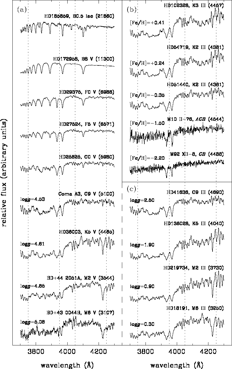Figure 3: Sample spectra of stars observed in run 6. Effective temperatures are given in parenthesis. Panel a) is a sequence in spectral types for main sequence stars. Panel b) shows stars with similar temperature but with a wide range in metallicity. Panel c) displays a sequence in spectral types for giant stars, which can be compared with the lower part of the dwarf sequence in panel a)

  

Figure 4: D4000 as a function of $\theta\equiv 5040/T_{\rm eff}$ for the whole sample. Stars are plotted using the same code as in G93 or W94

(ii) Sky subtraction. Since the field giant and dwarf stars of the library are bright, the exposure times were short enough to neglect the effect of an anomalous subtraction of the sky level. However, most of the cluster stars are not bright, being necessary exposures times of up to 1800 seconds for the faintest objects. In addition, the observation of these stars, specially those in globular clusters, were performed with the unavoidable presence of several stars inside the spectrograph slit, which complicated the determination of the sky regions. In [12, Cardiel et al. (1995)] we already studied the systematic variations on the D₄₀₀₀ measured in the outer parts of a galaxy (where light levels are only a few per cent of the sky signal) due to the over- or under-estimation of the sky level. We refer the interested reader to that paper for details. Although there is not a simple recipe to detect this type of systematic effect, unexpectedly high D₄₀₀₀ values in faint cluster stars can arise from an anomalous sky subtraction.

(iii) Flux calibration. Due to the large number of runs needed to complete the whole library, important systematic errors can arise due to possible differences among the spectrophotometric system of each run. In order to guarantee that the whole dataset is in the same system, we compared the measurements of the stars in common among different runs. Since run 6 was the observing run with the largest number of stars (including numerous multiple observations) and with reliable random errors (see above), we selected it as our spectrophotometric reference system. Therefore, for each run we computed a mean offset with run 6, which was introduced when it was significantly different from 0 (using a t test). It is important to highlight that differences between a true spectrophotometric system and that adopted in this work may still be present. Therefore, we encourage the readers interested in the predictions of the present fitting functions, to include in their observations a number of template stars from the library to ensure a proper correction of the data.

5.3 Final errors

The comparison of measurements of the same stars in different runs also provides a powerful method to refine the random errors derived in Eq. (8). We followed an iterative method which consistently provided the relative offsets and a set of extra residual errors to account for the observed scatter among runs (see [10, Cardiel 1999] for details).

As mentioned before, the data sample was enlarged by including 43 stellar spectra from the [44, Pickles' (1998)] library. The random errors in the D₄₀₀₀ indices measured in this subsample were estimated from the residual variance of a least-square fit to a straight line using all the stars (except supergiants) with $T_{\rm eff}\gt 8400$ K (they follow a tight linear relation in the $D_{4000}-\theta$ plane). The typical error in Pickles' spectra was found to be 0.036.