3 Simulations

In order to point out the behaviour and robustness properties of the $\hat\gamma_{\rm L^2}$ and $\hat\gamma_{\rm Q}$ variogram estimators, we simulate a sinusoidal process

$$m(t_i)=0.1 \sin\left(\frac{2 \pi}{70} t_i \right)+\varepsilon_i,$$

where $\varepsilon_i$ is the noise, independently and identically distributed according to a Gaussian law $N(0,\sigma_{\rm noise}^2)$ with $\sigma_{\rm noise}=0.01$. The amplitude of the signal is set to 0.10 and the period to 70 days, a possible period for semi-regular red giant stars (Jorissen et al. 1997). This process is visualized in Fig. 4a. As we would like to come to a more realistic case, we generate the same behaviour but with the time sampling t_i taken from the star HIP 111771, which is taken as representative of the mission (although the sample is rather heterogeneous). This data set is shown in Fig. 4b and is used to compute the variogram with $\hat\gamma_{\rm L^2}$(Fig. 5a above) and $\hat\gamma_{\rm Q}$ (Fig. 5a below) respectively. Both estimators are able to detect the period around 70 days, given by the first significant minimum.

  

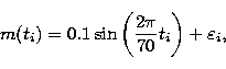
Figure 4: Simulated sinusoidal process with noise. a) regular time sampling, b) irregular time sampling for the star HIP 111771

  

Figure 5: Estimated variograms (above $\hat\gamma_{\rm L^2}$, below $\hat\gamma_{\rm Q}$) of the simulated sinusoidal process. a) without outlier, b) with one outlier

In order to show conspicuously the differences between the two estimators when the signal is perturbed by outliers, we took the previous simulated data and changed only one value. We put it at $5\sigma_{\rm signal}$ from the mean. Actually, this value can sometimes occur in real data from Hipparcos. The effect of the substitution of that single value can be seen in Fig. 5b, which should be compared with the Fig. 5a. Several remarks can be made. First, the $\hat\gamma_{\rm L^2}$estimator shows a flat and slight declining curve around the period: the signature of the periodicity has totally disappeared. In comparison, the general behaviour of $\hat\gamma_{\rm Q}$ has not changed. Second, the estimation of the micro-scale variability $\sigma^2_{\rm noise}$ jumped with $\hat\gamma_{\rm L^2}$. Furthermore, there is a higher jump at the second lag, which would suggest that there is some variability in the signal for extremely short time-scales. Again $\hat\gamma_{\rm Q}$ stays unchanged. With this example we see that $\hat\gamma_{\rm L^2}$ is not reliable when outlying values are present in the data, and that $\hat\gamma_{\rm Q}$ is more invariant to such values, i.e. $\hat\gamma_{\rm Q}$ is a highly robust estimate of the variogram.