2 Statistical analysis of periodicity for irregular sampling

There are many ways to describe periodic signals (Cuypers 1997). Most of the proposed methods are valid for rather strictly periodic signals: they are not very efficient when there is not a full conservation of the phase or of the amplitude. We may cite the following methods: "string" (Renson 1978), analysis of variances (Schwarzenberg-Czerny 1989), Fourier (Deeming 1975; Ferraz-Mello 1981; Babu & Feigelson 1996). Fortunately there are other methods which are better adapted to nearly periodic signals. The wavelets (Foster 1996), the autocorrelation (Bartholdi 1988; Edelson & Krolik 1988) methods and finally the structure function (Hughes et al. 1992), or variogram. These methods are obviously linked to each other. The last one is appropriate for our situation, as will be shown.

2.1 The variogram

In order to describe a pseudo-periodic signal, we introduce the concept of variogram. Let us consider a time series $\{m(t)$: $t\in D\}$, where D is a subset of ${\Bbb{R}}_+$. We can think of m(t) as the magnitude of a star at time t. Suppose that the signal m(t) can be decomposed into the sum of a deterministic part, $\mu(t)$, plus a stochastic part, the noise. Assume that this series satisfies the following hypothesis

$E\left(m(t)\right)=\mu(t),\quad \forall t\in D,$ (a)

Var$\left(m(t+h)-m(t)\right)=2\gamma(h),\quad \forall t,t+h\in D,$(b)

where $2\gamma(h)$ is the variogram, which can be used in practice in order to study the periodicity of the time series.

An interesting variogram that exhibits negative correlations caused by periodicity of the series is the wave (or hole effect) variogram (Cressie 1993) given by:

$$\gamma(h,a,b,c)=\left\{\begin{array} {ll} 0 & {\mathrm {if}... ...c}\right) \Big) & {\mathrm {otherwise,}} \end{array} \right.$$

where $a\geq 0$, $b \geq 0$ and $c\geq 0$. An example of a wave variogram is shown in Fig. 1. A hole effect shows oscillations of decreasing amplitude around the plateau called the sill, $a+b=\sigma_{\rm signal}^2$, which is the total variance of the time series. The oscillation reflects periodicity in the data and the first minimum is considered as a period or pseudo-period of the time series. The parameter a is usually called nugget effect and represents the micro-scale variability $\sigma_{\rm noise}^2$ due to measurement noise.

Note that a strictly periodic signal would show a periodic variogram defined by Journel & Huijbregts (1978):

$$\gamma(h,a,b,c)=\left\{\begin{array} {ll} 0 & {\mathrm {if}... ...h}{c}\right) \Big) & {\mathrm {otherwise,}}\end{array} \right.$$

where $a\geq 0$, $b \geq 0$ and $c\geq 0$. However, in practice, the oscillations are often dampened.

  

Figure 1: Wave variogram for a pseudo-periodic signal

2.2 The Matheron variogram estimator

Consider the series of differences at lag h defined by v(h)=m(t+h)-m(t). Let $\{m(t_1), ~\ldots,m(t_n)\}$ be a sample of a time series, and $\{v_1(h),~\ldots,v_{N_h}(h)\}$ be the corresponding sample of differences at lag h, where $N(h)=\{(t_i,t_j)$: $t_i-t_j=h\}$ and N_h is the cardinality of N(h). The classical variogram estimator proposed by Matheron (1962), based on the method-of-moments, is

$$2\hat\gamma_{\rm L^2}(h)=\frac{1}{N_h} \sum_{i=1}^{N_h} (v_i(h)-\bar v(h))^2, \quad h\in {\Bbb{R}}_+,$$

where $\bar v(h)=\frac{1}{N_h} \sum_{i=1}^{N_h} v_i(h)$. This estimator is based on the L² scale estimator (Genton & Rousseeuw 1995), which is unbiased, but behaves poorly if there are outliers in the data. One single outlier can destroy this estimator completely. For that reason, Genton (1998) proposed a highly robust variogram estimator.

2.3 The highly robust variogram estimator

In the context of statistical analysis of periodicity, variogram estimation is a crucial stage, because it determines the period or pseudo-period. Therefore, it is important to have a variogram estimator which remains close to the true underlying variogram, even if outliers (faulty observations) are present in the data. Experience from a broad spectrum of applied sciences shows that measured data may contain between 10 to 15 percent of outlying values (Hampel 1973) due to gross errors, measurement mistakes, faulty recording, etc. One might argue that any reasonable exploratory data analysis would identify outliers in the data. However, this approach may be subjective and informal. Furthermore, the existence of exploratory techniques does not supersede the usefulness of robust techniques. In this paper, we advocate the use of estimators which take account of all the available information in the data.

In the context of scale estimation, Rousseeuw & Croux (1992, 1993) have proposed a simple, explicit and highly robust estimator, called Q_Nh, which is defined by

$$Q_{N_h}=2.2191 \, \Big\{\vert v_i(h)-v_j(h)\vert;i<j\Big\}_{(k)},$$

where the factor 2.2191 is for consistency with the Gaussian distribution, $k={[N_h/2]+1 \choose 2} = ([N_h/2]+1)[N_h/2]/2$, and [N_h/2] denotes the integer part of N_h/2. This means that we sort the set of all absolute differences |v_i(h)-v_j(h)| for i<j and then compute its k-th order statistic (the first quartile for large N_h). This value is multiplied by the factor 2.2191, thus yielding Q_Nh. Note that this estimator computes the k-th order statistic of the ${N_h \choose 2}$ interpoint distances. This estimator is shown to be very robust to outliers in the data. It is of interest to remark that Q_{N<<609>> h} does not rely on any location knowledge and is said to be location-free. The estimator Q_{N<<610>> h} can be computed using no more than ${\it O}(N_h \log N_h)$ time and ${\it O}(N_h)$ storage, by means of the fast algorithm described in Croux & Rousseeuw (1992).

Using the previous definitions, Genton (1998) defines a highly robust variogram estimator as

$$2\hat\gamma_{\rm Q}(h)=(Q_{N_h})^2,$$

and discusses its use and properties.

2.4 Variogram estimation for irregularly spaced data

  

Figure 2: Diagram of pairwised differences. a) regular time sampling, b) irregular sampling for the star HIP 111771

Structure functions are used in AGN studies (Hughes et al. 1992). Apparently this goes well with the signals they want to study, because they are mainly interested in the slope of the rising curve of the structure function which gives information in the frequency domain (Paltani 1996). However for periodic signals, the oscillations may be diminished in their analysis. We are left with the difficulty of the choice of the binning and of the width of the bins. A too narrow width would have the disastrous effect to have too little measurements in a bin, whereas a constant binning can be too large for short periods and smears out the periodic behaviour. This is the reason why we choose to have a binning linked with the period investigated. Denote by

$$2\gamma_{\rm b}(h)=\frac{1}{2f(h)}\int_{h-f(h)}^{h+f(h)} 2 \gamma(u){\rm d}u,$$

the binned variogram based on a lag function f. It is natural to require for a time-scale invariant variogram, i.e. $2 \gamma_1(h)=2 \gamma_2(ah)$, a>0, that the binned variogram be invariant too. This is achieved by choosing the linear lag function $f(h)=\delta h$, as is shown by One has to determine the fraction $\delta$, in order to get an optimal binning of the variogram. If data would be regularly spaced, one could let $\delta \rightarrow 0$, and use the classical method $2\gamma_{\rm b}(h)=2\gamma(h)$. Figure 2 depicts the diagram of pairwised differences for regularly and irregularly (HIP 111771 time sampling) spaced data. A closer look at Fig. 2 indicates that if the period is h, we should set $\delta < 1/2$, otherwise too much information about the period is lost. Therefore, a good compromise between regularity and period information is to let $\delta=1/4$.

  

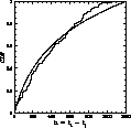
Figure 3: Empirical cumulative distribution function (CDF) of the lag differences for the star HIP 111771, and logarithmic approximation F(h) (smooth line) of the empirical CDF

The remaining problem is the choice of the lags, i.e. the position of the bin location. If one chooses equidistant lags, there would be too many bins for large lags, and too few for small lags. Therefore, the distribution of the lags is a crucial question. Figure 3 represents the empirical cumulative distribution function (CDF) of the lags of the star HIP 111771, and indicates that a logarithmic scale of the lags

$$F(h)=\log\left(\frac{9}{1200}h+1\right)$$

is a satisfactory approximation. Other stars have also been analysed and the same approximation can be used for most of them. Note that the greatest available lag is h=1200, and we set F(0)=0 and F(1200)=1. In consequence, we adopt the choice of lags $h_0,~\ldots,h_{k}$ such that $F(h_0),~\ldots,F(h_{k})$ are equidistant on the interval [0,1]. The number k of lags must be chosen such that a good temporal resolution is achieved (for instance, k=90 is a typical value with Hipparcos time sampling).

Another approach in the choice of the lags consists in computing quantiles of the empirical distribution of each star. The advantage of this method is its adaptability to the particular sampling of each star, whereas the former one was global. Moreover, lags are defined only when new data points are present. The drawback is that it provides clumped bin locations.