5 Simulation method and results

 In this section, the myopic deconvolution performance is studied. In order to show the influence of the turbulence noise on the deconvolution process and the gain brought by a myopic regularization, a very partial AO correction has been simulated as following.

We have considered an AO system operating on a D = 3 m telescope with a 1 m central obstruction diameter. The turbulence is characterized by a single layer with a Fried parameter equal to 10 cm at the imaging wavelength $\lambda = 0.5~ \mu$m, a ${\bar v} = 20$ m/s wind velocity. The AO system is made up of a $9 \times 9$ Shack-Hartmann wavefront sensor, and a 88 piezo-stack mirror. The servo-loop bandwidth is 80 Hz. The simulation tool used was developed at ONERA (Rousset et al. 1991). 1024 instantaneous phase screens are simulated. Each wavefront gives a short exposure PSF. The sample frequency (500 hz) leads to a total integration time of 2 seconds. With such a short integration time, the turbulence noise is not negligeable. In these conditions, and for a 11.5 magnitude object (corresponding to 55 detected photons per sub-aperture and per frame), we obtain a very partial correction characterized by its PSF with a Strehl ratio of 0.03 (ratio between the intensity at the center of the corrected PSF and the intensity of the diffraction limited PSF).

${\tilde h}_{\rm m}$ is directly deduced from the simulated wavefronts using Eq. (6). Note that, in this case, we have an ideal measurement of the residual wavefront and therefore an ideal estimation of ${\tilde h}_{\rm m}$.

The STF is computed by the average of the 1024 square moduli of the short exposure OTFs. The PSD is therefore deduced from Eq. (7).

The corrected image of a binary star, including photon noise, is shown in Fig. 1 (10⁶ detected photons in the whole image). We consider a $128\times 128$ image sampled at the Nyquist frequency, i.e. with a pixel angular size $\frac{\lambda}{2D} = 0.033 \ \rm arcsec$ (field of view = $4.2 \ \rm arcsec$).

  

Figure 1: AO corrected image of a binary star (simulation with Strehl ratio equal to 0.03). Total flux 106 photons, only photon noise in the image

The separation of the two components is $\Delta {\rm sep} = 10.4$ pixels, i.e., an angular separation of $0.34 \ \rm arcsec$. The intensity of two components are $7.153\ 10^5$ and $2.847\ 10^5$ photons i.e., a magnitude difference equal to $\Delta m = 1$.

The image presented in Fig. 1 clearly shows the need of a deconvolution process for the estimation of the star positions and magnitudes.

A pixel-by-pixel deconvolution (no reparametrization of the object) gives good results (Conan et al. 1997; Mugnier et al. 1998), but the star positions are known only within a pixel and the photometry measurement is not very accurate because of the residual flux in the background after deconvolution. The multiple-star object model avoids both of these limitations. Note, however, that the number of stars is assumed to be known. In practice, this number may be difficult to estimate from the long exposure image, in particular in low Signal to Noise Ratio (SNR) conditions. In this case, it is possible to perform a two step deconvolution process: a pixel-by-pixel deconvolution to estimate the number of star and a "multiple-star object model'' deconvolution to improve the astrometry and the photometry. The ultimate performance, in case of very low flux SNR, are currently being investigated. A more sophisticated scheme would involve the simultaneous detection of the number of stars and the estimation of their parameters (Champagnat et al. 1996).

Comparison beetwen pixel-by-pixel and reparametric deconvolution are presented in (Mugnier et al. 1998). In the following, one will focus on the reparametric deconvolution and especially the gain brought by a myopic deconvolution.

Table 1 shows the statistics of the deconvolved parameters over 50 different photon noise realizations. The results are obtained by processing the image with the following techniques:

• a crude estimation (value and position of the two maxima in the image)
• a classical deconvolution. The first term of the criterion defined in Eq. (5) is minimized assuming that PSF is constant and equal to $h_{\rm m}$.
• a blind deconvolution. The sole first term of the criterion defined in Eq. (5) is minimized with respect to the object parameters and PSF (i.e., no PSF regularization)
• a myopic deconvolution, as presented above (the sum of all terms of Eq. (5) are minimized).

  

Table 1: Simulation results: $<\Delta{\rm sep}\gt$ and $\sigma_{\Delta{\rm sep}}$ are the average and the standard deviation of the separation (pixel unit and arcsecond unit) between the two components calculated on 50 different noise realizations. $<\Delta I\gt$ and $\sigma_I$ are the average and the standard deviation of the global error between the true and estimated intensities of the two components in photon unit. They are calculated on 50 different noise realizations ($\Delta I = 100\sqrt{\vert\alpha_1-\alpha_{\rm 1 es}\vert^2+\vert\alpha_2-\alpha_{\rm 2 es}\vert^2}/(\alpha_1+\alpha_2)$). Recall that 1 pix = $\frac{\lambda}{2D}$ = 0.033 arcsecond

It shows that a deconvolution and especially a myopic deconvolution method increases the accuracy of the parameter estimation.

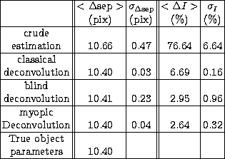The classical deconvolution gives a very good result on the star separation: a sub-pixel precision, no bias and an accuracy (standard deviation) about 66 times lower than the diffraction limit $\left(\frac{\lambda}{D}\right)$. Nevertheless, the problem of the classical deconvolution lies in the deficiency of the flux estimation ($\simeq 7 \%$). This error is mostly due to a bad restitution of the global flux ($\alpha_1+\alpha_2$) which is a free parameter in the deconvolution process. This evolution may be important to take into account the possible loss of flux in the image, due to stars bordering the field of view.

The introduction of the myopic deconvolution leads to better photometric results (a better restitution of the global flux). The error on $\alpha_{\rm 1es}$ and $\alpha_{\rm 2es}$ is significantly reduced ($2.64 \%$).

The separation estimation, which is already good for the classical case is not improved by the myopic one. The accuracy is even slightly lower than in the classical case $\left({\rm about}\ \frac{\lambda}{50 D}\right)$ but it is not significant. The good estimation, obtained here in the classical case, is most likely due to the fact that the mean PSF is a good estimate of the simulated PSF (circular symmetry, no static aberrations, only turbulent noise) and is good enough for the estimation of the separation. Yet, the accuracy of the star positions should be increased by the myopic deconvolution in the case of a badly estimated PSF.

The blind deconvolution, which is not regularized, is markedly less stable than the myopic one, in the sense that estimated object parameters are more dependent on the noise outcomes on the image (important increase of the standard deviations) and are consequently less accurate.

In short, the classical deconvolution is good enough for an astrometric estimation, but the myopic deconvolution is needed to improve the object photometry (by a factor 3.5 in our case). As described below, it also leads to a better PSF estimation. A good PSF determination is important because the myopic deconvolution is a joint estimation on the object and the PSF. Therefore, an accurate PSF restitution leads to an accurate estimation of the object parameters.

  

Figure 2: Cut off normalized Optical Transfer Function versus spatial frequency: true AO corrected OTF (dashed-dotted line), mean OTF (dashed line), Blind deconvolved OTF (dotted line) and Myopic deconvolved OTF (solid line) are shown for comparison. The spatial frequency is normalized to the telescope cutoff frequency. The photon noise level $\frac{1}{{\bar N}}$ is indicated for comparison

Figure 2 shows a cut of the different normalized OTF. It shows that a blind or a myopic deconvolution improves the accuracy of the OTF at low frequencies (where the signal to noise ratio is high). But the blind deconvolution is limited by the photon noise. The noise has been propagated, and amplified, from the image to the estimated PSF (the expected behavior in a non-regularized case).

On the other hand, the myopic deconvolution allows a better restitution of the PSF even at high frequencies, and avoid the noise propagation and amplification.

  

Figure 3: Circular average of the modulus of the difference between: true OTF and mean OTF (dashed line), true OTF and Blind deconvolved OTF (dotted line), true OTF and Myopic deconvolved OTF (solid line). The photon noise level $\frac{1}{{\bar N}}$ is indicated for comparison

Figure 3 allows a frequency to frequency assessment of the gain brought by the myopic deconvolution on the PSF. The influence of the regularization is visible at high frequencies, where the myopic deconvolved OTF follows the mean OTF and decreases below the photon noise level.

The average distance between the true PSF and its different estimations, $<\sqrt{\vert PSF_{\rm true} - PSF_{\rm est}\vert^2}\gt$, is a good summary of the Figs. 2 and 3 and quantifies the gain brought by the myopic deconvolution on the PSF:

• distance between the true and the mean PSF: $2.72\ 10^{-5}$.
• average and standard deviation of the distance between the true and the blind deconvolved PSF: $2.22 \pm 0.08\ 10^{-5}$
• average and standard deviation of the distance between the true and the myopic deconvolved PSF: $1.05 \pm 0.03\ 10^{-5}$.

The values are given for a unit energy PSF.

The simulations have shown that, in the case of very partial AO correction (ie a strong turbulent noise), a myopic deconvolution increases the accuracy of the joint estimation on the object parameters and the PSF. It leads, in particular, to good photometry estimation.