3 The myopic deconvolution method

It is well-known that image restoration is an ill-posed problem which needs to be regularized through the use of additional a priori information (Tikhonov & Arsenin 1977), and (Demoment 1989) for a review.

The goal of myopic deconvolution is to restore both the object and the PSF knowing the image intensity measurements and the a priori information.

We model our observed object (field of stars) by a sum of Dirac functions (Gunsay & Jeffs 1995). Its intensity is then given by:  

$$o(\vec{r}) = \sum_i^n{\alpha}_i\delta(\vec{ r}-\vec{a}_i)$$ (2)

where $\vec{a}_i$ and $\alpha_i$ are the position vector and the intensity of the $i{\rm th}$ star respectively and are the object parameters we are seeking. We consider that n, the number of stars, is a known parameter.

A constant or slowly variable parameter can also be added to account for sky background and underlying emission (Lucy 1994).

The deconvolution method we use is based on a stochastic approach i.e., we consider object parameters and PSF as outcomes of stochastic processes (Conan 1998).

Bayes' rule combines the likelihood of the data with the a priori distribution of the parameters (object and PSF, which are decorraleted processes) into the a posteriori probability distribution of the unknowns ($\vec{ a}_i, \alpha_i$ and h):  

$$p(\vec{ a}_i,\alpha_i,h\vert d) \propto p(d\vert\vec{a}_i,\alpha_i,h)\times p(\vec{ a}_i,\alpha_i)\times p(h)$$ (3)

where p(A|B) means conditional probability of A given B.
$p(d\vert\vec{ a}_i,\alpha_i,h)$ corresponds to the noise probability law (likelihood term) and accounts for the noise affecting the image: photon and detector noise. In a first approximation we choose a stationary white Gaussian statistics for the noise probability, although a non-stationary gaussian or poisson plus gaussian statistics would be more accurate.

$p(\vec{ a}_i,\alpha_i)$ reflects the a priori knowledge (or prior) on the object parameters. In addition to the reparametrization itself, which contains a strong constraint on the object, we also use:

• the positivity of the star intensities, enforced in our case by a reparametrization of intensities by magnitudes. $\alpha_i = 10^{-0.4*m_i}$ where m_i is the star magnitude.
• an upper limit on the star intensities
  ($\sum_i\alpha_i<{\rm whole\ image\ flux}$).

Similarly, p(h) reflects the a priori knowledge on the PSF. It can be reasonably assumed to be Gaussian and is therefore characterized by its first and second moments (Conan et al. 1998): a mean PSF ($h_{\rm m}$) and a Power Spectral Density [PSD] ($PSD_{\rm h}$). This PSD can be viewed as a per frequency variance of the Optical Transfer Function [OTF] (Fourier Transform of the PSF) around its mean value.

The method used to calculate $h_{\rm m}$ and $PSD_{\rm h}$ using the Wave-front sensor (WFS) data or the image of a reference star will be described in Sect. 4.

Following the Maximum A Posteriori (MAP) approach, a set of estimated parameters is given by the maximization of $p(\vec{ a}_i,\alpha_i,h\vert d)$, the a posteriori probability law:  

$$[\hat{\alpha_i},\vec{ {\hat a}}_i, {\hat h}] _{\rm map} = {\r... ...max}_{\alpha_i,\vec{ a}_i,h} [p(\vec{a}_i,\alpha_i,h\vert d)].$$ (4)

In this case, maximizing the probability corresponds to minimizing the following criterion ($-\log{p(\vec{a}_i,\alpha_i,h\vert d)}$) in the Fourier domain:

$$\begin{eqnarray} J(\alpha_i,\vec{ a}_i,{\tilde h}(\vec{ f})) \!\!&=&\!\!\sum_{\... ...ec{ f})-{\tilde h}_{\rm m}(\vec{ f})\vert^2}{PSD_{\rm h}(\vec{f})}\end{eqnarray}$$ (5)

where $\tilde .$ denotes a Fourier transform, N² the pixel number, $\sigma^2$ the noise variance and $\vec f$ the spatial frequency.

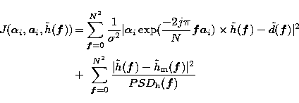
The first term of Eq. (5), is the likelihood term which takes into account the object reparametrisation.

The second term is a regularization term on the PSF. It draws the actual OTF towards its mean value ${\tilde h}_{\rm m}$ with a stiffness related to its PSD. This term avoids a noise propagation and amplification on the PSF (cf. Sect. 5) as well as the trivial solution (PSF = image and all the sources = 0 except one delta function).

This leads to a strong decrease of the number of parameters. In the case of a $128\times 128$ pixels image of a binary star, the number of parameters drops from 16384 (if the object parameters are the intensity on each pixel) to 6 (two intensities, two position vectors). It therefore allows a better precision on these parameters; in particular, a sub-pixel determination of star position -- meaning a fraction of $$\frac{\lambda}{2D}$$ for Shannon sampled images -- and an accurate photometry measurement.
Also, fewer parameters to estimate lead to a faster convergence.

We now turn to the different ways of estimating the PSF and its associated PSD.