3 Limitations and problems

 

3.1 Variation in $\Omega$

The approximations employed in this algorithm are valid for accurate work in many applications, but there are certain classes of orbit for which the approximations break down and may lead to inaccurate results.

First, and perhaps most importantly, the algorithm assumes a fixed inclination between the two orbital planes. In reality, the angle $\Omega$ changes with time and this results in a change of the mutual inclination $\Delta i$.

In order to deal with this we repeatedly use the fixed plane algorithm and integrate across the distribution of $\Delta i$ produced by the variations of $\Omega_1$ and $\Omega_2$. The integration is carried out over the variable $\Delta \Omega$, the difference between $\Omega_1$ and $\Omega_2$, using standard one-dimensional methods over the interval $\Delta \Omega = (0, 2\pi)$.

It is easy to show that $\Delta i$ is a simple function of $\Delta \Omega$ such that  

$$\cos{\Delta i} = \cos{i_{1}} \cos{i_{2}} + \sin{i_{1}} \sin{i_{2}} \cos{\Delta\Omega}$$ (20)

assuming that i₁ > i₂.

Taking this into account, it becomes possible to cover the vast majority of orbits, but there remain small regions of configuration space where the algorithm breaks down due to geometric singularities. These singularities do not exist in the real system and arise only as a result of the simplified encounter geometry, namely the approximation of rectilinear relative motion during the close encounter.

3.2 Variation in other elements

The algorithm assumes that the elements a, e and i are so slowly varying that they can be assumed to be constant over timescales of interest. In some instances this may not be the case, particularly if the objects are affected by secular perturbations that significantly affect (for example) the eccentricity and inclination, even in cases when the semi-major axis is approximately constant. The point has been discussed by Davis et al. (1992), and in principle such variations could be accommodated within the present algorithm by adding further layers of integration to the model. However, this removes the virtues of simplicity and speed from the model, and would require a more complete dynamical representation of the system. If exact results are required in particular cases, then it may be necessary to return to a computer-intensive numerical integration scheme.

3.3 Singularities

It is likely that in any application involving a large number of test bodies some pairs of orbits will lie sufficiently close to singular regions to produce unrealistic results. Singularities are also encountered with other methods, since they are implicit in the assumptions on which the algorithm is based.

Inaccurate results will be produced by pairs of orbits with low relative inclinations, and indeed Öpik suggested that his theory was inadequate for inclinations $<1^{\circ}$. The value of $\Delta \omega$ approaches infinity, at least as evaluated by the simple equations, since as $\Delta i$ approaches zero it becomes impossible to separate the orbits by rotating them around the origin. Examination of the conditions makes it clear that the maximum value of $\Delta \omega$ should be smaller than the size of the phase space over which we are integrating.

The simplest way to prevent this is to ensure that the relative inclination used during the integration is never less than some critical value. The adjustment of the relative inclination should be performed on the inclinations of the input orbits, rather than by limiting $\Delta i$,shifting the values of i₁ and i₂ such that Eq. (20) will give a value higher than our enforced limit for all values of $\Delta \Omega$.

Similarly, problems occur when the perihelia or aphelia of either orbit coincide, since for such orbits the separation parameter $S\rightarrow 0$ at this point and therefore $\Delta \omega$diverges. This is a direct result of approximating the curved trajectories in space at the close encounter by straight lines. For orbits with configurations sufficiently close to this singularity condition the results will be inaccurate.

In the version of the code implemented by the authors these singularities are dealt with by interpolating across the region where the singularity is known to exist. Orbits with q or Q sufficiently close to the Q or q of the other have probabilities computed by taking variations of each orbit with slightly differing elements, the magnitude of these variations being chosen to be comparable to the short-term variations in the orbital elements introduced by ordinary planetary perturbations. In practical applications we have found that such an approach produces reasonable results.

We emphasize that these singularities, arising from nearly coplanar or tangent orbits, are unphysical, in the sense (as proved by Wetherill 1967) that the corresponding collision integrals are always finite and can in principle be evaluated using other methods. One way of dealing with them is to use a more appropriate numerical integration technique, as was implemented by Farinella & Davis (1992); another, involving a suitable change of coordinates to remove the improper integral, has been discussed by Milani et al. (1990). In either case, owing to orbital evolution, the singularities are only short-lived, and the method of handling them has to be considered in relation to the physics of the dynamical system.

3.4 Uniformity of sampling within $(\omega_{1},\omega_{2})$-space

The present algorithm assumes that the orbits sample $(\omega_{1},\omega_{2})$-space uniformly. It is difficult to provide simple rules to determine whether a pair of orbits satisfies this criterion adequately. For example, both orbits may be in resonances, leading the orbit pairs to have strongly correlated elements. Such orbits may only explore certain regions of phase space, along specific paths, and we can no longer logically assume that every point in $(\omega_{1},\omega_{2})$-space is equally likely. Obviously, for every pair of orbits the evolution of $\omega_1$ and $\omega_2$ can in principle be determined, but good pairs will explore most of $(\omega_{1},\omega_{2})$-space uniformly. The approximation to this behaviour is that every point in $(\omega_{1},\omega_{2})$-space is equally weighted, as too are the points on the curve of intersection. Unfortunately, the most straightforward way to avoid these difficulties is through a direct numerical integration of the problem orbits, which of course is computationally expensive and is what this and similar methods have been designed to avoid.

3.5 Gravitational focusing

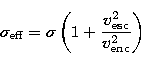
The algorithm assumes fixed target radii, but if the bodies have sufficient mass then the effective target area will be a function of their relative velocity, owing to their mutual gravitational attraction. For spherical targets with a combined mass M=M₁ +M₂ and radius of interaction R=R₁+R₂ the effective cross section, $\sigma_{\mbox{\scriptsize eff}}$ can be calculated from

$$\sigma_{\mbox{\scriptsize eff}} = \sigma \left(1+\frac{v_{\mbox{\scriptsize esc}}^2}{v_{\mbox{\scriptsize enc}}^2}\right)$$ (21)

where $v_{\mbox{\scriptsize enc}}$ is the relative encounter velocity, $\sigma$ is the unfocused cross section (i.e. $\sigma = \pi (R_1+R_2)^2$), and $v_{\mbox{\scriptsize esc}}^2 = 2GM/R$. This correction must be applied at each point of the sampled curve, since the relative velocity is a function of $(\omega_{1},\omega_{2})$.

We note that both P (proportional to $\Delta t$) and $\Delta \omega$are proportional to R, so the resulting collision probability is proportional to R² and therefore proportional to $\sigma$.