4 Results and discussion

In this paper we present the observational results and the primary qualitative conclusions. In a future paper we will present a quantitative discussion of the results.

4.1 The radio spectra

The flux densities are presented in Tables 4 and 5 and plotted in Figs. 1 to 5.

  

Figure 1: Radio spectra of the objects of the complete sample

  

Figure 2: Radio spectra of the objects of the complete sample

  

Figure 3: Radio spectra of the objects of the complete sample

  

Figure 4: radio spectra of the additional objects

  

Figure 5: radio spectra of the additional objects

  

Table 4: Polarization for the complete sample

  

Table 5: Polarization of additional objects

In order to extract information from the radio spectra, we fitted them with a hyperbola (which is a curve tending asymptotically to a straight line at the extrema). We first fit the spectral indices in the thick and thin part of the spectrum independently, and then fixed these two values (which correspond to the angular coefficients of the asymptotes) and we performed a least square fit, solving for the other parameters of the hyperbola.

We calculated the frequency of the spectral peak (Tables 1 and 2) using the fitted curves. We show the distributions of the observed and rest frame turnover frequency for the 33 sources of the complete sample in Figs. 6c and 6d. In Figs. 6a and 6b we show the high frequency (above the peak) and low frequency (below the peak) spectral index distribution, respectively.

4.2 The spectral indices and the turnover frequency

The GPS radio sources are a mixed group of galaxies and quasars, with some remarkable differences between the two classes. The histogram in Fig. 16a shows that the redshift distribution is very different for galaxies and quasars. The galaxies have a typical redshift of $\sim$0.5, and none has a redshift higher than 1. For the galaxies without redshift information, we note that only 0316+161 has an optical magnitude slightly fainter than the galaxy 2128+048 at redshift 0.99 (Table. 1). Since these galaxies follow the Hubble diagram (O'Dea et al. 1996; Snellen et al. 1996) it is unlikely they will be found at a redshift much higher than the others in the sample. The quasars are instead found at any redshift (we included the galaxy 1404+286 (OQ208), which has a Seyfert 1 nucleus, in the quasar class) with the majority at very high z (see also O'Dea 1990).

  

Figure 6: Histograms for the complete sample: a) high frequency spectral index distribution; b) low frequency spectral index distribution; c) observed turnover frequency distribution; d) rest frame turnover frequency distribution

The high frequency spectral index ranges from 0.5 (the limit set in the selection criteria) to 1.3 with the galaxies having perhaps slightly steeper values (but the 2 objects with the steepest spectral indices are quasars). The low frequency spectral index ranges from -0.2 to -2.1 without any clear difference between galaxies and quasars, but the higher values are biased since in several objects the low frequency part of the spectrum is under-sampled and the spectral index is calculated close to the turnover frequency where it is likely to be flatter. Similar results were found by De Vries et al. (1997) though their poorer frequency coverage resulted in a somewhat smaller range in spectral index.

The quasars tend to peak at higher frequencies than the galaxies in both the rest frame and observed frame and some quasars have a turnover frequency in their rest frame exceeding 10 GHz. This suggests that, on the assumption that the turnover is caused by synchrotron self-absorption, the GPS quasars are more compact than the galaxies. This effect has been also found by De Vries et al. (1997) in a bright heterogeneous sample and by Snellen (1997) in a fainter sample. In addition, VLBI images of several sources belonging to the complete sample show that quasars are more compact than galaxies, and in general exhibit different morphologies (Stanghellini et al. 1997).

These results suggest that either GPS galaxies and GPS quasars are different types of objects, or that beaming of compact components plays a role in the quasars (see also O'Dea 1998).

4.3 Extended emission

  

Figure 7: 0248+430 at 1.35 GHz. The restoring beam is 1.41 $\times$ 1.32 arcsec in PA $-78^\circ$. The rms noise on the image is 0.2 mJy. The peak flux is 810 mJy/beam. The contour levels for all the images are -3, 3, 6, 12, 25, 50, 100, 200, 500, 1000 $\times$ the rms noise

  

Figure 8: 0528+134 at 1.66 GHz. The restoring beam is 1.14 $\times$ 1.01 arcsec in PA $+2^\circ$. The rms noise on the image is 0.25 mJy. The peak flux is 2088 mJy/beam

We have detected extended emission (both diffuse and compact) close to the compact radio source in some cases at 21 cm. In the remaining sources, our upper limits on extended emission is typically 1 mJy/beam at 21 cm.

0248+430 (Fig. 7) has a compact emitting region 15 arcsec east of the main component and a hint of weak emission 5 arcsec to the south. 0528+134 is resolved, showing an extension in the NW direction (Fig. 8). Murphy et al. (1993) present an image of 0738+313 at 20 cm showing 2 emitting regions resembling 2 weak hot-spots and lobes on the opposite sides of the dominant component. In our image (Fig. 9) these 2 weak components are almost completely resolved out and only a hint of emission has been detected 30 arcsec north and south of the compact region. 0941-080 shows a slightly resolved secondary component 20 arcsec east of the main one (Fig. 10). 2134+004 has very weak and diffuse emission around the strong compact component (Fig. 11). 2223+210 has a secondary component 4 arcsec away from the main one in the SW direction in our image at 1.35 GHz (Fig. 12); the main component itself is resolved in a core-jet structure oriented NE with a possible counter jet in the image at 5 GHz (Fig. 13). 2230+114 at 1.35 GHz (Fig. 14) shows an elongated structure in the NW-SE direction with a hint of emission bending to SW, while in the 4.9 GHz image (Fig. 15) the elongated structure turns out to be a core-jet structure with the possible presence of a counter jet.

Stanghellini et al. (1990) report several cases of extended emission around GPS radio sources. Of the objects presented here showing extended emission, 0528+134 and 2223+210 are not true GPS objects (see also Sect. 4.4 for a discussion of the case of 0528+134). In a couple of sources (0248+430, 0941-080 both belonging to the complete sample) it is difficult to say whether the secondary emission is related to the GPS radio source and further observations are probably needed. The extended emission found around 0738+313, 2134+004, and 2230+114 (the first 2 objects belong to the complete sample) is likely to be related to the GPS object. In the complete sample, 0108+388 is known to have extended emission, so there are 3 to 5 objects out of 33 with known extended emission so far. This percentage of 9 to 15$\%$ is slightly smaller but consistent with that previously claimed by Stanghellini et al. (1990). It is clear that the vast majority ($\sim 90\%$)of the GPS sources appear to be truly isolated and have no emission beyond the kpc scale at the current limits.

4.4 Variability

Waltman et al. (1991) presented monitoring observations at 2.7 and 8.1 GHz for several GPS sources covering the time range from 1979 to 1988. Some sources as 0237-233, 1245-197, 1345+125 were found to be very stable in flux density. Others were found to be variable: 0552+398 shows a variation of $\sim$30% at 8.1 GHz. 2134+004 has a variability of about 15 - 20$\%$at 8.1 GHz. 2352+495 has a variability below 10$\%$ at 8.1 GHz. Also 0742+103 is slightly variable.

Wehrle et al. (1992) also report variability for some GPS objects in the time range 1985-1991 at 4.8, 8, and 14.5 GHz, from the University of Michigan Radio Astronomy Observatory monitoring program for several sources, some of which are GPS objects. 0552+398 shows an increase in flux density exceeding 50$\%$ at 8.4 and 14.5 GHz, 1127-145 shows a quasi periodical variability of approximately 1 Jy at all the 3 frequencies. The source 2230+114 also shows a rather remarkable flux density variability at all the 3 frequencies with an amplitude of 0.5 - 1 Jy and is a well known low frequency variable source (Bondi et al. 1996). The variability of 1404+286 has been discussed by Stanghellini et al. (1996).

In conclusion, we find that some GPS sources (mainly quasars) show mild to high flux density variability at cm and mm wavelengths. However, without uniform monitoring of the complete sample it will not be possible to determine how common this variability is. We also note a couple sources where the spectral shape is variable and at some times the spectrum was peaked, and at other times it was not, 0528+134, the well known gamma-ray source (Mukherjee et al. 1996), and 0201+110. Both of these sources show a rather flat spectrum in the VLA observations from the second or the third session and they would be very easily discarded as GPS radio sources. But 0528+134 has been included in the class of GPS radio sources because of its GPS-like spectrum from the literature (O'Dea et al. 1991), and 0201+113 really shows a convex spectrum in the data in the first VLA session published in O'Dea et al. (1990). This behavior is not surprising in highly variable radio sources as we may well expect that the presence of new radio components will change the spectral shape. Thus, there are sources which show a peaked spectrum only part of the time. This aspect of the GPS phenomenon deserves more attention as it could be related to the remarkably different properties found between GPS galaxies and (some?) GPS quasars.

  

Figure 9: 0738+313 at 1.33 GHz. The restoring beam is 2 $\times$ 2 arcsec. The rms noise on the image is 0.3 mJy. The peak flux is 1943 mJy

  

Figure 10: 0941-080 at 1.33 GHz. The restoring beam is 2.44 $\times$ 1.54 arcsec in PA $+29^\circ$. The rms noise on the image is 0.5 mJy. The peak flux is 2088 mJy/beam

  

Figure 11: 2134+004 at 1.33 GHz. The restoring beam is 1.91 $\times$ 1.55 arcsec in PA $-5^\circ$. The rms noise on the image is 0.4 mJy. The peak flux is 3249 mJy/beam

  

Figure 12: 2223+210 at 1.33 GHz. The restoring beam is 1.37 $\times$ 1.32 arcsec in PA $-7^\circ$. The rms noise on the image is 0.3 mJy. The peak flux is 1663 mJy/beam

  

Figure 13: 2223+210 at 5 GHz. The restoring beam is 0.37 $\times$ 0.35 arcsec in PA $+5^\circ$. The rms noise on the image is 0.3 mJy. The peak flux is 1034 mJy/beam

  

Figure 14: 2230+114 at 1.33 GHz. The restoring beam is 1.46 $\times$ 1.36 arcsec in PA $+1^\circ$. The rms noise on the image is 0.8 mJy. The peak flux is 6444 mJy/beam

  

Figure 15: 2230+114 at 5 GHz. The restoring beam is 0.38 $\times$ 0.36 arcsec in PA $-11^\circ$. The rms noise on the image is 0.5 mJy. The peak flux is 4137 mJy/beam

  

Figure 16: Histograms for the complete sample: a) redshift distribution; b) fractional polarization at 1.3 GHz; c) fractional polarization at 4.9 GHz; d) fractional polarization at 8.5 GHz

4.5 Polarization

Due to the low level of observed polarization, the errors are dominated by the rms noise on the polarization images (typically 0.5 mJy) and by contamination from residual unpolarized emission (estimated about $0.2-0.3\%$ of the total flux density). The error in the polarized flux may then be calculated as $\sigma _{\rm P}=\sqrt {0.5^2 + (0.003\times S_{\rm mJy})^2}~{\rm mJy}$.We considered any measurement of the fractional polarization below 0.3$\%$ to be an upper limit (Tables 6 and 7). The errors in the position angle have a systematic contribution due to the uncertainty in the determination of the position angle of the calibrator (3C 286), assumed to be around 2-3 degrees. This is the dominant contribution in the position angle error for most of the objects with detected polarized flux density.

In Fig. 16 we show the histograms of the fractional of polarization (mostly upper limits) for the complete sample at 1.3, 4.9 and 8.5 GHz. The fractional polarization is in general low at all the frequencies. Only a few quasars have a fractional polarization above 1% at 4.9 or 8.5 GHz.

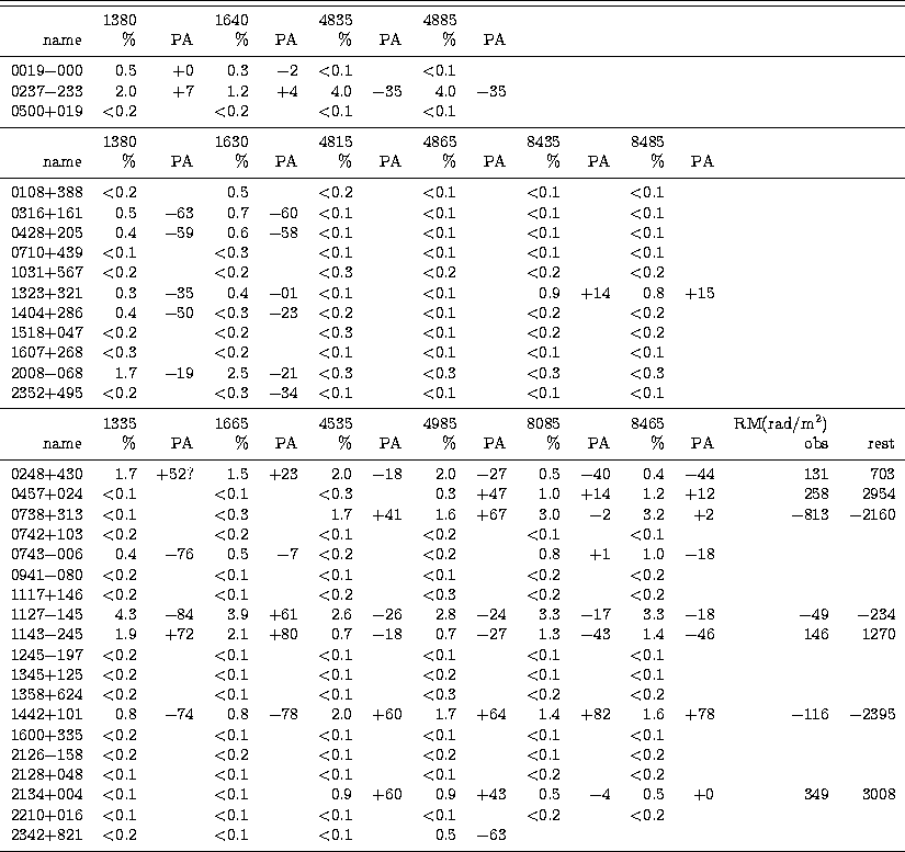
When polarized emission has been detected we attempted a linear fit to the polarization angles versus the squared observed wavelength, as is expected from the Faraday effect on polarized radiation propagating through a magnetized and ionized medium.

The low level or even the lack of detection of polarized flux limited us to only a few sources (all quasars). The fits are generally rather good and are given in Tables 6 and 7, and in Figs. 15 and 16. Due to the better frequency coverage in the present observations, our estimated rotation measures supersede those reported by O'Dea et al. (1990), though we cannot rule out that some of the difference is due to variability. We find Faraday rotation measures in the rest frame above 1000 rad/m² for 5 quasars of the complete sample. We also found a very high value (>10⁴ rad/m²) for 0552+398 which does not belong to the complete sample but has a GPS shape.

Sometimes the frequencies which give a good fit include those close to the turnover, and in the case of 0552+398 are all below the turnover. This implies that the region emitting the polarized emission is different from that responsible for the optically thick emission or that the turnover is not caused by synchrotron self absorption.

4.6 Summary and conclusions

We have presented a bright flux-density-limited complete sample of 33 GPS radio sources selected on the basis of their peaked radio spectra. The sample selection was based on observations with the VLA, WSRT, and other instruments. Additional GPS sources not belonging to the complete sample have also been observed. We present our results on the polarization and radio spectrum. We found remarkable differences in the properties of quasars and galaxies, the latter having lower turnover frequencies, mostly undetectable polarization and lower redshifts.

In the few objects where polarization has been detected at many frequencies, the Faraday rotation measure in the rest frame often exceeds 1000 rad/m².

In about 10% of the sources we detect weak diffuse extended emission. In the remaining $\sim 90\%$ any extended emission has a peak surface brightness is less than about 1 mJy/beam at 21 cm.

In a following paper we will discuss the implications of the properties of the complete sample in the framework of the scenarios proposed to explain the existence of the GPS radio sources.

Acknowledgements

We thank Ger de Bruyn for advice on the reduction of the WSRT observations and Wim De Vries for comments on the manuscript. C.S. wishes to thank the STScI Collaborative Visitor Program for providing support for his visits. The VLA is operated by the U.S. National Radio Astronomy Observatory which is operated by Associated Universities, Inc., under cooperative agreement with the National Science Foundation. The Westerbork Synthesis Radio Telescope is operated by the Netherlands Foundation for Research in Astronomy (NFRA) which is financially supported by the Netherlands organization for scientific research (NWO) in the Hague. We have made use of the NASA/IPAC Extragalactic Database, operated by the Jet Propulsion Laboratory, California Institute of Technology, under contract with NASA.