3 Data reduction

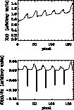
The following step is the determination of the position of the lunar edge in each image and then the correlation between the images of the same frame. The edge is found column by column introducing a coordinate, x, and a function, I(x), proportional to the intensity of the pixels in that column (see Fig. 4(above)). It is assumed that the edge of the Moon produces an intensity leap higher than any other feature in the image (except for the cut due to the edge of the CCD):

  

Figure 4: Intensity plot in arbitrary units (above) and its derivative (below) along one column of the CCD

the pixel with the highest slope is then the value of x in which the derivative $\partial I(x) / \partial x$, reaches its maximum (see Fig. 4(below)). In order to find with better accuracy the position of the edge within the pixel, this one and the two pixels at its sides are fitted with a parabola.
We have made extensive tests in laboratory with illumination conditions similar to the one experienced during the run and we can say that the vertex of the parabola allows one to determine the position of the edge with a repeatability of approximately 0.07 arcsecs.

Every edge, obtained at a time t, is then represented by a vector of 192 elements, $[x_{(1,t)},\dots,x_{(192,t)}]_i$, with $i=1,\dots,s$,and every frame containing s images is reduceded to a matrix of s rows, each row corresponding to an edge. Rows of the same matrix are scaled in order to have the same value in the first element, that is equivalent to say:

$$x_{(1,t)_1}= \dots = x_{(1,t)_i} = \dots = x_{(1,t)_s} .$$ (3)

The standard deviation between the s rows, column by column, is then calculated moving along the edge, for $j=1,\dots,192$:

$$\sigma_j = \sqrt{{1 \over s} \sum_{i=1...s} \left( x_{(j,t)_i} - \bar{x}_{(j,t)} \right) ^2} ,$$ (4)

and this is equivalent to measuring the loss of correlation in the atmospheric induced tilt perturbations as the distance from a reference point increases.

  

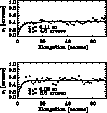
Figure 5: Interpolating the data allows to obtain both the values for $\theta_0$ and for r0. It can be seen the loss of correlation between tilt perturbations for increasing distances from a reference point along the edge of the Moon. These are two examples of the data collected during the tests. Only one portion of the field of view, the most interesting, is plotted

Forcing all the edges in the same image to have the same value in the first pixel, introduces a multiplicative factor, $\sqrt 2$, that has to be considered when determining the value of $\sigma_j$.The multiplicative factor arises because the variance of the first pixel, $\sigma_1^2$, sums quadratically with the absolute variance of each other pixel, $\sigma^2_{\rm abs}$, that is equivalent to say:

$$\sqrt{\sigma^2_1+\sigma^2_{\rm abs}} = \sqrt{2\sigma^2_{\rm rel}}\,.$$ (5)

Plotting the standard deviation versus the distance from the reference position this loss of correlation is clearly visible (see Fig. 5). In these examples, over a distance of the order of less than 5 arcsec, the correlation is completely lost and the data show statistical oscillations around a mean value, $\sigma_\theta$.This residual scatter is due both to Poissonian statistic, because of the limited number of edges collected in each image, to the photometric noise (including read out and photon shot noise) and finally to inhomogeneities in sensitivity of the pixels.

In order to find the value of $\theta_0$, that is the value for which the correlation decreases of a factor ${\rm e}^{-1}$,we fitted the data with the following function:

$$f(\theta) = \sqrt{2} \sigma_\theta \left[1- \exp \left( -{\theta \over \theta_0 } \right) \right].$$ (6)

However, it can be noted from one of the data plots, that this is only a rough approximation of the expected theoretical behaviour (Valley & Wandzura 1979).

In fact, sometimes one can observe at moderate angular distances an anticorrelation between the tilt perturbations and this is due to the fact that what is measured is not just the tilt component but instead it is the sum of both tilt and coma of any order.

Although we did not measure the anticorrelation because we had not enough samples to obtain a reliable estimate, it must be noted that knowing the amount of anticorrelation can be used to have a comparison between the observed turbulence power spectrum and that of Kolmogorov.

When the anamorphic relay is used to increase the size of the field of view it is possible, in principle, to increase the precision in the measurement of $\theta_0$ within the same image. In fact one can choose to have as a reference point not only one of the pixels at the edges of the CCD but also one or more pixels in the center of the field, more distant from each other than the isokinetic angle.

Finally, considering the observed tilt effect on the rigid movement of the elongate LGS to be of the same order of that introduced in Eq. (1) one can recover (with the same equation but changing $D_{\rm p}$ from the diameter of the laser projector to the diameter of the seeing monitor) the characteristic value of r₀ for the night during which the tests where performed.