3 Practical considerations

It is now worthwhile to highlight a number of practical considerations with respect to the actual implementation of the SCIDAR technique.

3.1 Effect of finite spatial and temporal sampling

The theory outlined in Sect. 2.3 assumes an infinitely small spatial and temporal scintillation detection sampling rate. Obviously, however, for the practical implementation of SCIDAR one has to compromise the level of detectable scintillation for the sake of obtaining a reasonably high signal-to-noise level in the detected intensity. Consequently our choice of spatial and temporal sampling means that the level of scintillation detected will be less than that inferred by the theory, leading to an underestimate of C_n²(h). This may explain, for example, some of the relatively high values of r₀ we obtain - as shown in Sect. 4. For the relatively low sampling rates used in our system ($\Delta r \simeq 1$ cm pix^-1 and $\Delta t = 1.6$ or 2.7 ms) this underestimate could be corrected, to first order, by linearly-calibrating our results with respect to the integrated C_n²(h) value determined by other means during the observations. This feasibility is planned for our purpose-built SCIDAR system currently under construction.

3.2 Signal-to-noise considerations

At any particular time during an observation run a number of binary star objects may be available for the collection of SCIDAR data. Therefore an obvious consideration one first has to make is regarding the signal-to-noise trade-off between various potential targets. Given the magnitudes of each component for a number of potential targets, one can calculate the error propagation for the expression involving B₁ and B₁ in the second term of Eq. (10) to predict the relative average signal-to-noise ratio (SNR) with respect to photon noise.

  

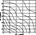Figure 7: Contour plot of the relative SNR for various binary star magnitude combinations. Contours are at 10% the peak level. The values decrease from left to right

Figure 7 shows such a calculation for a typical range of values encountered in practice and enables one therefore to make an informed choice.

However, if one is collecting data across the whole telescope pupil using a telescope with a large obstruction ratio, one also has to take into account the effect of the pupil transfer function upon the SNR within the correlation plane. This is particularly so if one is operating in the generalised SCIDAR mode since one is then imaging the scintillation pattern viewed through two overlapping pupils. The degree of pupil overlap is directly proportional to both the angular separation of the binary and the effective distance below the telescope pupil one defocuses to.

  

Figure 8: Example transfer functions of overlapping pupils, for the generalised SCIDAR case, as a function of altitude. Curves are given for binary star separations of 2, 4, 6 & 8 arcseconds and assume a telescope diameter of 1 m and 1 cm pix-1 image plane sampling

Figure 8 shows the predicted pupil overlap transfer function for various binary separations assuming a 1 m telescope pupil of obstruction ratio 0.3 and a typical defocus distance of 3.5 km. As can be seen in the most extreme case, for example beyond separations of 8 arcseconds, the distorted transfer function can significantly reduce the SNR for high altitudes.

3.3 C_n²(h) altitude resolution

Since close to zenith, $\Delta h = \Delta r/\theta$, in theory one is free to choose whatever altitude sampling length is required. However, for a particular telescope diameter D, in practice a restriction is imposed by the requirement that the maximum height attained should be greater than the sum of the height for which optical turbulence is assumed to be negligible and the magnitude of the generalised SCIDAR conjugate plane distance, $\vert h_{\rm conj}\vert$, ie: $h_{\rm max}$ = D/$\theta \geq$ 20 km + $\vert h_{\rm conj}\vert$.

These restrictions upon binary star separation are shown graphically in Fig. 9 for an assumed pupil sampling of 1 cm pix^-1, a telescope pupil diameter of 1 m and a conjugate plane distance of 3.5 km.

  

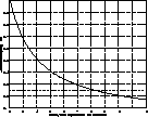Figure 9: Plot of altitude resolution as a function of binary separation showing the limits imposed for a reasonable altitude sampling (top) and a maximum altitude reached of 25 km above image plane (bottom), for a 1 m telescope assuming 1 cm pix-1 image plane sampling

Taken in combination, the restrictions implied in Fig. 8 and Fig. 9 show that for this particular configuration, binary separations between around 4-7 arcseconds are desirable.

It must be noted that both the upper limit upon $\theta$ and the SNR within the correlation plane can be increased, if using a telescope of a large enough diameter (e.g. D > 3.5 m) to enable an artificial circular pupil greater than 1m to be imposed within the image of the segment of the mirror observed. In this case, assuming a similar pupil sampling as previously, the restriction upon $\theta$ then only originates from the size of the CCD, such that in our case $\theta < 11''$.

3.4 Estimating the error on C_n²(h)

Having calculated a solution C_n²(h) profile from the data, one also requires some knowledge of the reliability of this solution. Although this is difficult to ascertain directly when using the iterative maximum entropy routine (Sect. 2) due to the non-linear nature of the iterative procedure, it has been found that it is possible to estimate the RMS error of a solution using a numerical approach.

To enable this we define a ``solution plane", which contains both the true (and unknown) $C_{n\rm ~true}^{2}$ profile and the best-fit solution profile, $C_{n\rm ~best-fit}^{2}$, and a ``data plane", within which resides both the true (observed) data, $A\rm _{data}$, and the correlation function obtained from the $C_{n\rm ~best-fit}^{2}$ profile, $A\rm _{best-fit}$.
A schematic outline of this representation is shown in Fig. 10.

  

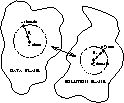Figure 10: Schematic description of the method used to estimate the RMS error on any particular Cn2(h) profile obtained

Given that one can then represent the RMS difference ${\cal E}_{\rm A}$given by Eq. (15), as the geometrical distance in the data plane between $A\rm _{data}$ and the final $A\rm _{best-fit}$, what one wishes to find is the corresponding distance between $C_{n\rm ~true}^{2}$ and $C_{n\rm ~best-fit}^{2}$, namely ${\cal E}_{\rm C}$ - as indicated in Fig. 10.

The approach taken here is to numerically perturb the $C_{n\rm ~best-fit}^{2}$ profile about its position within the solution plane by incremental distances by applying random Gaussian noise, until the RMS distance within the data plane between its corresponding correlation function and $A\rm _{data}$ is equal to the RMS distance ${\cal E}_{\rm A}$. When this occurs the RMS distance between $C_{n\rm ~best-fit}^{2}$ and its perturbed value can then be considered as describing the radius of a circle within the solution plane upon which the ``true" value of C_n²(h) lies and therefore represents a reasonable approximation of the RMS error ${\cal E}_{\rm C}$.

In doing so one is assuming that the solution $C_{n\rm ~best-fit}^{2}$ is close to the global minimum within the solution plane, or at least within a local minimum which is not very different from the true solution. This assumption is justified both by the relatively low value of ${\cal E}_{\rm A}$ we achieve prior to termination of the iterative routine and also by the strongly linear relationship that has been found in all cases between ${\cal E}_{\rm A}$ and ${\cal E}_{\rm C}$ as the degree of perturbation applied to $C_{n~\rm best-fit}^{2}$ is increased.

Having performed this calculation for a number of different C_n²(h) profiles, it has been found that the value of ${\cal E}_{\rm C}$ is greater than the value of ${\cal E}_{\rm A}$ in most cases. For example for the case shown in Fig. 5, ${\cal E}_{\rm A}$ and ${\cal E}_{\rm C}$ are found to be 4.3% and 7.2% respectively. This highlights the need for high SNR data for a reliable C_n²(h) solution.