Simulations can be used for deriving the probability that a wavelet coefficient is not due to the noise (Escalera et al. 1992). Modeling a sky image (i.e. uniform distribution and Poisson noise) allows determination of the wavelet coefficient distribution and derivation of a detection threshold. For substructure detection in a cluster, the large structure of the cluster must be first modeled, otherwise noise photons related by the large scale structure will introduce false detections at lower scales. If we have a physical model, Monte Carlo simulations can also be used (Escalera & Mazure 1992; Grebenev et al. 1995), but this approach requires a long computation time, and the detections will always be model-dependent. Damiani et al. (1996), and also Freeman et al. (1996) propose to calculate the background from the data in order to derive the fluctuations due to the noise in the wavelet scales. It is regretable to have to do this, because we lose one the main advantage of the use of the wavelet transform, which is to be background-free. Indeed, wavelet coefficients have a null mean, and the detection is just done by comparison to a given threshold. Furthermore, background estimation is not an easy task, and generally requires several steps (filtering, interpolation, etc), and error estimation on the background is generally difficult to calculate.
A straightforward method, initially proposed by (Bijaoui & Giudicelli 1991),
for deriving the detection levels
at each scale is to apply a sigma clipping at each scale.
Therefore a standard deviation ![]() is
estimated at each scale j, and wavelet coefficients wj(x,y)
are considered as significant if
is
estimated at each scale j, and wavelet coefficients wj(x,y)
are considered as significant if
![]()
where k is generally taken equal to 3. This method allows us to easily
detect strong features, but is certainly not optimal for detection of weak
objects. Indeed, as the noise is not Gaussian, it is
difficult to estimate the real probability of false detection
using this ![]() detection criterion.
detection criterion.
Vikhlinin et al. (1995) proposed to assume a Gaussian
local noise, and to estimate the map ![]() from the
the local background. The standard deviation
from the
the local background. The standard deviation ![]() related to a wavelet coefficient wj(x,y) is derived from
related to a wavelet coefficient wj(x,y) is derived from
![]() using the property of linearity of the wavelet
transform (Starck & Bijaoui 1994). As previously, the hypothesis
is not true, and the consequence is the same. A solution
is to use Monte Carlo simulations to set the correspondence between
the standard deviation of a wavelet coefficient and the levels
of significance (Grebenev et al. 1995), but the
simulations must be performed for each image because the significance
levels vary strongly with the number of photons (Grebenev et al. 1995).
using the property of linearity of the wavelet
transform (Starck & Bijaoui 1994). As previously, the hypothesis
is not true, and the consequence is the same. A solution
is to use Monte Carlo simulations to set the correspondence between
the standard deviation of a wavelet coefficient and the levels
of significance (Grebenev et al. 1995), but the
simulations must be performed for each image because the significance
levels vary strongly with the number of photons (Grebenev et al. 1995).
In Slezak et al. (1994) and
Biviano et al. (1996), the Anscombe transform
![]()
has been used and acts as if the data arose from a Gaussian
noise with white model, with ![]() , under the assumption
that the mean value of I is large. Simulations have shown
(Murtagh et al. 1995) that a number of photons less than
30 per pixel introduces a bias. In X-ray images, the number of
photons is often lower, and sometimes can even be equal to zero.
Using Anscombe transform in this case will introduce an over
estimation of the noise level. To overcome this difficulty,
the noise standard deviation can be reestimated, for instance
as in (Slezak et al. 1994) i.e. by applying a sigma
clipping at the first scale of the wavelet transform. However,
this approach assumes that the noise is homogeneous,
which is not true. Indeed, if the number of photons per pixel
is lower that 30, the standard deviation of noise after
Anscombe transformation, is varying strongly with the number
of photons (Murtagh et al. 1995).
, under the assumption
that the mean value of I is large. Simulations have shown
(Murtagh et al. 1995) that a number of photons less than
30 per pixel introduces a bias. In X-ray images, the number of
photons is often lower, and sometimes can even be equal to zero.
Using Anscombe transform in this case will introduce an over
estimation of the noise level. To overcome this difficulty,
the noise standard deviation can be reestimated, for instance
as in (Slezak et al. 1994) i.e. by applying a sigma
clipping at the first scale of the wavelet transform. However,
this approach assumes that the noise is homogeneous,
which is not true. Indeed, if the number of photons per pixel
is lower that 30, the standard deviation of noise after
Anscombe transformation, is varying strongly with the number
of photons (Murtagh et al. 1995).
An approach for very small numbers of counts, including frequent zero cases, has been described in Slezak et al. (1993) and Bury (1994), for large scale clustering of galaxies. We have adopted here the same approach to analyze X-ray images.
A wavelet coefficient at a given position and at a given scale j is
![]()
where K is the support of the wavelet function ![]() (i.e. the box in which
(i.e. the box in which
![]() is not equal to 0) and nk is the
number of events which contribute to the calculation of wj(x,y) (i.e. the
number of
photons included in the support of the dilated wavelet centered at (x,y)).
is not equal to 0) and nk is the
number of events which contribute to the calculation of wj(x,y) (i.e. the
number of
photons included in the support of the dilated wavelet centered at (x,y)).
If a wavelet coefficient wj(x,y) is due to the noise, it can be considered
as a realization of the sum ![]() of
independent random variables
with the same distribution as that of the wavelet function (nk
being the number of photons or events used for the calculation of wj(x,y)).
Then we compare the wavelet coefficient of the data to the values
which can taken by the sum of n independent variables.
of
independent random variables
with the same distribution as that of the wavelet function (nk
being the number of photons or events used for the calculation of wj(x,y)).
Then we compare the wavelet coefficient of the data to the values
which can taken by the sum of n independent variables.
The distribution of one event in the wavelet space is directly
given by the histogram H1 of the wavelet ![]() . Since
independent events are considered, the distribution of the random variable
Wn (to be associated with a wavelet coefficient) related to n
events is given by n autoconvolutions of H1
. Since
independent events are considered, the distribution of the random variable
Wn (to be associated with a wavelet coefficient) related to n
events is given by n autoconvolutions of H1
![]()
Figure 1 (click here) shows the shape of a set of Hn. For a large
number of events, Hn converges to a Gaussian.
![]()
Figure 1: Autoconvolution histograms for the wavelet associated with a
B3 spline scaling function for 1 and 2 events (top left), 4 to
64 events (top right), 128 to 2048 (bottom left), and 4096 (bottom
right)
In order to facilitate the comparisons, the variable Wn of distribution
Hn
is reduced by
![]()
E being the mathematical expectation,
and the cumulative distribution function is
![]()
From Fn, we derive ![]() and
and ![]() such
that
such
that ![]() and
and ![]() .
.
Let us define a reduced wavelet coefficient as
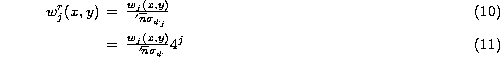
where ![]() is the standard deviation of the wavelet function,
is the standard deviation of the wavelet function,
![]() is the standard deviation of the dilated wavelet function
(
is the standard deviation of the dilated wavelet function
(![]() ), and wj(x,y) a wavelet coefficient
obtained using the à trous wavelet transform algorithm.
), and wj(x,y) a wavelet coefficient
obtained using the à trous wavelet transform algorithm.
Therefore a reduced wavelet coefficient, wrj(x,y), calculated from
wj(x,y), and resulting from n photons or counts is significant if:
![]()
or
![]()
This detection method presents several advantages: it is independent of any model, no simulation is needed, and it is theoretically rigorous.