![]()
The choice of ![]() is based on an a priori knowledge of the
behavior of the solution. For each value t of the time, one defines an
"index" function
is based on an a priori knowledge of the
behavior of the solution. For each value t of the time, one defines an
"index" function ![]() mapping
mapping
![]() on [1,n]; the shell with the index 1 (respt. n)
corresponds to the center (respt. to the top of the envelope).
Therefore the integration is made on an equidistant grid.
In terms of the derivative of Q with respect to q:
on [1,n]; the shell with the index 1 (respt. n)
corresponds to the center (respt. to the top of the envelope).
Therefore the integration is made on an equidistant grid.
In terms of the derivative of Q with respect to q:
![]()
Eq. (16 (click here)) becomes:
![]()
Note that Q is a linear function of q as soon as the
Eqs. (17 (click here)) and (18 (click here)) are fulfilled.
The change of variables ![]() gives:
gives:
![]()
where:
![]()
can be derived from the analytic form of ![]() .
Thus, there are two more unknowns:
.
Thus, there are two more unknowns:
![]() and
and ![]() ; they fulfill a system
of differential equations of first order with boundary conditions:
; they fulfill a system
of differential equations of first order with boundary conditions:
![]()
here ![]() is computed by Eq. (15 (click here)) with
the value of
is computed by Eq. (15 (click here)) with
the value of ![]() obtained at the bottom of the atmosphere.
The set of equations to be solved on the
equidistant grid,
obtained at the bottom of the atmosphere.
The set of equations to be solved on the
equidistant grid, ![]() is therefore:
is therefore:
The initial and boundary conditions are straightforwardly
expressed in terms of q. Note that the
derivative, with respect to time, of the specific internal energy and of the density
should be taken along directions d![]() , i.e., d
, i.e., d![]() , taking
into account the change of mass due to the mass defect.
Indeed, the solution, by the damped Newton Raphson scheme, of the non-linear
Eq. (21 (click here)), necessitates the knowledge
of the derivatives of
, taking
into account the change of mass due to the mass defect.
Indeed, the solution, by the damped Newton Raphson scheme, of the non-linear
Eq. (21 (click here)), necessitates the knowledge
of the derivatives of ![]() ,
, ![]() and U, with
respect to the mass, taking into account the changes of chemical composition;
that is the more restrictive conditions imposed by the use of this automatic
allotment of mesh points; it is also a consequence of the fact that the
integro-differential problem,
Eq. (1 (click here)), cannot be solved as a whole since,
along the evolution, convective zones appear, disappear, cede or recede with
not fixed limits.
Moreover with an equidistant mesh in q, differences between close numbers
are avoided; that is particularly sensitive in the external part of
the envelope where the changes of mass between two
adjacent grid points are very small.
and U, with
respect to the mass, taking into account the changes of chemical composition;
that is the more restrictive conditions imposed by the use of this automatic
allotment of mesh points; it is also a consequence of the fact that the
integro-differential problem,
Eq. (1 (click here)), cannot be solved as a whole since,
along the evolution, convective zones appear, disappear, cede or recede with
not fixed limits.
Moreover with an equidistant mesh in q, differences between close numbers
are avoided; that is particularly sensitive in the external part of
the envelope where the changes of mass between two
adjacent grid points are very small.
Q should be a strictly monotonous, two times differentiable,
function, and as simple as possible. By experiments,
it has been found![]() that:
that:
![]()
is, in all, the most convenient form; for the two "distribution factors"
![]() and
and ![]() , the heuristic values:
, the heuristic values:
![]()
are close to those used by Eggleton (1971). The function
![]() can now be explicitly calculated using Eq. (19 (click here))
and Eq. (21 (click here)).
In the core, the pressure gradient is not large and the mesh refinement is
monitored by the changes of
can now be explicitly calculated using Eq. (19 (click here))
and Eq. (21 (click here)).
In the core, the pressure gradient is not large and the mesh refinement is
monitored by the changes of ![]() , i.e., the mass; while, in the outermost part of
the envelope the repartition function is controlled by the changes of
, i.e., the mass; while, in the outermost part of
the envelope the repartition function is controlled by the changes of ![]() , i.e.,
the pressure, due to its large gradient; there, from a grid point to the next,
the mass changes are very small, typically
, i.e.,
the pressure, due to its large gradient; there, from a grid point to the next,
the mass changes are very small, typically ![]() ,
even
,
even ![]() , while for, the pressure, the changes are of
the order of
, while for, the pressure, the changes are of
the order of ![]() (with
(with ![]() , see next paragraph); a similar
situation occurs on the neighborhood of shell sources.
, see next paragraph); a similar
situation occurs on the neighborhood of shell sources.
Between a PMS initial model and an evolved model at the beginning of the
4He burning, the central pressure is magnified by more than
30, that also affects the distribution constant C(t); the accuracy is ensured
whatever the age is, if the repartition constant, is kept almost fixed with
respect to time; that is done by increasing (or decreasing)
the total number of shells in such a way that C(t) remains within ![]() , of its initial value. With
, of its initial value. With ![]() ,
, ![]() and
and
![]() , the relative change in pressure within a shell is typically
10% and the number of zones in a PMS initial solar model is of
the order of 250, it increases to
, the relative change in pressure within a shell is typically
10% and the number of zones in a PMS initial solar model is of
the order of 250, it increases to ![]() at present solar age and more
than
at present solar age and more
than ![]() at the onset of the helium flash.
at the onset of the helium flash.
In that case, ![]() and
and ![]() ;
; ![]() and
and ![]() , are derived from Eq. (8 (click here)) with
, are derived from Eq. (8 (click here)) with
![]() and
and
![]() .
The Rosseland mean opacity
.
The Rosseland mean opacity ![]() is a function of density and
temperature, therefore the non-linear
system of Eq. (23 (click here)) must be solved by iterations for
is a function of density and
temperature, therefore the non-linear
system of Eq. (23 (click here)) must be solved by iterations for ![]() ,
,
![]() ,
, ![]() and for their derivatives with respect to
and for their derivatives with respect to ![]() and
and ![]() .
.
As described in Sect. 2.4.3, the precise reconstitution of an atmosphere consists
in a differential problem, with boundary conditions at three different levels:
![]() ,
, ![]() and
and ![]() ;
recall that, at
;
recall that, at ![]() , defined by Eq. (10 (click here)), there is a
open inner limit; the solution given to this numerical challenge is described
in Appendix B3.
, defined by Eq. (10 (click here)), there is a
open inner limit; the solution given to this numerical challenge is described
in Appendix B3.
Similarly, for the eulerian variables, one defines:
![]() and
and
![]() .
Equations, initial and boundary conditions are straightforwardly derived.
.
Equations, initial and boundary conditions are straightforwardly derived.
Due to (i) the splitting in two steps of the integration of the whole problem, and (ii) to the ability of restoring the solution at any point, a grid can be especially designed for the chemicals; this net is refined in the inner parts (recall that thermonuclear reaction rates have a high power law dependence with respect to the temperature) where the nuclear reactions are active.
As noticed previously, a long-lasting discontinuity on chemical composition is
an unphysical situation; therefore, when the diffusion is ignored, if no
physical process is explicitly introduced, the discontinuities are smoothed by
the
numeric, the lower the order of the numerical scheme is, the more efficient is
the smoothing. Satisfactory results have been obtained
using, for a given time step, the mass points designed for the quasi-static
problem, and for the next time step, mass points located at half distance
between two neighbouring mass points designed for the quasi-static
problem; ensuring, however, that the
mass step, for the chemical composition is, at least, greater than
![]() , except for each CZ where a minimum of 10
points is required.
As far as a convective core increases, the chemicals undergo discontinuities at
its limit, while, when it recedes, at any point localized in the zone between
the
previous and the new limits of the core, the values of abundances not only
depend on the local temperature and density but, also, on how long that
point has lasted in the mixed receding core; a similar situation occurs as
soon as a
MZ recedes from a radiative zone. Moreover in radiative zones, when the
diffusion is
ignored, though violating the physics, the
discontinuities in chemicals formally stay so far they are not, again,
embedded in a new extent of a convective zone. It
is difficult to mimic in details and precisely all these tricky processes.
In CESAM,
the abundances at any point localized between the limit of a core and its
location at the former time step, are obtained by linear
interpolation, with respect to
, except for each CZ where a minimum of 10
points is required.
As far as a convective core increases, the chemicals undergo discontinuities at
its limit, while, when it recedes, at any point localized in the zone between
the
previous and the new limits of the core, the values of abundances not only
depend on the local temperature and density but, also, on how long that
point has lasted in the mixed receding core; a similar situation occurs as
soon as a
MZ recedes from a radiative zone. Moreover in radiative zones, when the
diffusion is
ignored, though violating the physics, the
discontinuities in chemicals formally stay so far they are not, again,
embedded in a new extent of a convective zone. It
is difficult to mimic in details and precisely all these tricky processes.
In CESAM,
the abundances at any point localized between the limit of a core and its
location at the former time step, are obtained by linear
interpolation, with respect to ![]() , between their values at the new and at the
previous locations of
the limit.
, between their values at the new and at the
previous locations of
the limit.
In the radiative zones, without diffusion, the equations to
be solved are written:
![]()
In MZ, the chemical composition is homogeneous and the equations for the mean
abundances can be written (see Sect. 2.3.1 (click here)):
therefore it is an integro-differential problem.
Another numerical difficulty results from large ratios between the
characteristic evolutionary time scales involved;
they can be estimated by the ratio between the eigenvalues, ![]() and
and ![]() , of minimum and maximum norms of the jacobian
matrix:
, of minimum and maximum norms of the jacobian
matrix:
![]()
Typically, with the physical conditions at
the center of the present Sun, ![]() K,
K, ![]() g cm-3,
one has:
g cm-3,
one has:
![]()
Such differential problems are called "stiff"
(Gear 1971; Hairer & Wanner 1991); special algorithms have been
developed for
their numerical solution; they ensure numerical stability even if the
time step is larger than the smallest characteristic time scale. However,
it is not possible to have accurate solution
for all the variables, regardless of the size of the time step;
therefore, owing to the stability of the scheme, the numerical
errors are damped out, a given accuracy being ensured for variables of interest.
Furthermore, chemical abundances being positive numbers, oscillations around
zero (as observed with the trapezoidal rule) are unsatisfactory.
The so-called "L-stable" schemes (Hairer & Wanner, loc. cit.)
have good stability properties without oscillations; they are suitable
for the integration of the evolution of chemicals abundances.
Equations (27 (click here))
and (28 (click here)) and their numerical counterparts are non-linear; they
are also implicit, as the L-stable schemes are.
The L-stable Implicit Runge Kutta (IRK) Lobatto IIIC
formula with orders![]() p=1, 2 and 4 are available in CESAM;
their coefficients are reproduced Table 5 (Appendix B4), p=1 is the standard
Euler's backward scheme (Hairer & Wanner, loc. cit.).
For the Lobatto IIIC formulas with order p greater than two, values for
the
temperature and density are needed at intermediate time levels. They are
estimated by interpolations of order four from successive models.
p=1, 2 and 4 are available in CESAM;
their coefficients are reproduced Table 5 (Appendix B4), p=1 is the standard
Euler's backward scheme (Hairer & Wanner, loc. cit.).
For the Lobatto IIIC formulas with order p greater than two, values for
the
temperature and density are needed at intermediate time levels. They are
estimated by interpolations of order four from successive models.
The comparison of solutions given by two IRK formula
which differ by one order of accuracy, i.e., the so-called Fehlberg method
(Stoer
& Bulirsch
1979), allows an estimate ![]() of the numerical accuracy.
Here the IRK formulas Radau IIA (Hairer & Wanner, loc. cit., Sect. IV.8)
are used in connexion with Lobatto IIIC formulas.
Let
of the numerical accuracy.
Here the IRK formulas Radau IIA (Hairer & Wanner, loc. cit., Sect. IV.8)
are used in connexion with Lobatto IIIC formulas.
Let ![]() be the value required for the relative precision; an
optimal value
be the value required for the relative precision; an
optimal value ![]() for the next time step is written:
for the next time step is written:
![]()
here p is the order of the IRK formula.
It has been observed that the robustness of the scheme is improved if
only small changes for the time step are allowed for; therefore the estimate of
the new time step ![]() is taken as:
is taken as:
![]()
This precise control of the numerical accuracy, practically, doubles the
computing time; it is prohibitive in most cases, therefore the time step is
simply adjusted in such a way that the
changes of the abundances remain within fixed limits
![]() .
.
With diffusion, for every ![]() (
(![]() ), the set of equations to be
solved is written:
), the set of equations to be
solved is written:
![]()
for ![]() .
As seen Sect. 2.3.1 (click here), the mixing in MZ is made by turbulent
diffusion. Since Eq. (30 (click here)) holds everywhere, the evolution
of the chemical composition is no longer an integro-differential problem but a
differential problem with
boundary conditions given by Eq. (7 (click here)) and Eq. (12 (click here)); it is a mixed
parabolic/hyperbolic problem.
At each LMR, the abundances Xi and the fluxes Fi are continuous
functions
with discontinuous first derivatives owing to the jumps of
.
As seen Sect. 2.3.1 (click here), the mixing in MZ is made by turbulent
diffusion. Since Eq. (30 (click here)) holds everywhere, the evolution
of the chemical composition is no longer an integro-differential problem but a
differential problem with
boundary conditions given by Eq. (7 (click here)) and Eq. (12 (click here)); it is a mixed
parabolic/hyperbolic problem.
At each LMR, the abundances Xi and the fluxes Fi are continuous
functions
with discontinuous first derivatives owing to the jumps of ![]() (see
Sect. 2.3.1 (click here)).
The method of integration of the diffusion equation, written in finite-elements
form, is described in Appendix B5.
(see
Sect. 2.3.1 (click here)).
The method of integration of the diffusion equation, written in finite-elements
form, is described in Appendix B5.
Figure 1 (click here) plots, with respect to the mass fraction, the
relative differences in
sound velocity for two calibrated solar models calculated,
respectively, with standard mixing and mixing by
diffusion (![]() ,
, ![]() and vi=0,
and vi=0,
![]() ).
The differences, at the level of 10-5, show the similar efficiency of
both approaches.
Figure 2 (click here) plots, with respect to the radius fraction,
the normalized abundances of 2D, 3He, 7Li, 7Be, 12C at the
onset of
the main sequence for a non-standard solar model, evolved from PMS,
including microscopic diffusion according to Michaud & Proffitt (1993);
at that age (45 My) the convective core of the young Sun recedes, while the CZ
is close to its present day location. One emphasizes on the well marked
drop of the gradient of 2D and on the smooth profile of 7Li at
the limit of the
CZ; due to the mixing, in the
convective core, the elements have a constant abundances except 8Be
since its nuclear time is of the order of the mixing time (
).
The differences, at the level of 10-5, show the similar efficiency of
both approaches.
Figure 2 (click here) plots, with respect to the radius fraction,
the normalized abundances of 2D, 3He, 7Li, 7Be, 12C at the
onset of
the main sequence for a non-standard solar model, evolved from PMS,
including microscopic diffusion according to Michaud & Proffitt (1993);
at that age (45 My) the convective core of the young Sun recedes, while the CZ
is close to its present day location. One emphasizes on the well marked
drop of the gradient of 2D and on the smooth profile of 7Li at
the limit of the
CZ; due to the mixing, in the
convective core, the elements have a constant abundances except 8Be
since its nuclear time is of the order of the mixing time (![]() 100 days). As
seen, the
Petrov-Galerkin's solution is stable even with strong jumps of more than
thirteen decades in the diffusion coefficients profiles.
100 days). As
seen, the
Petrov-Galerkin's solution is stable even with strong jumps of more than
thirteen decades in the diffusion coefficients profiles.
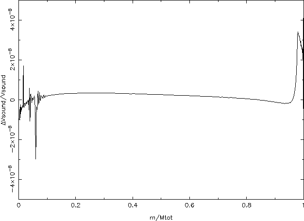
Figure 1: Relative difference of the sound velocity
between two calibrated solar models
calculated with the two kinds of mixing: standard instantaneous mixing and
diffusion. The low level of the differences shows that the two kinds of mixing
have similar effects. The wiggly behavior for radius lesser than
![]() is a fossil signature of the discontinuities of
chemicals at the limit of the convective core of the young sun; they are
almost not smoothed because these calculations employed a low
dissipative scheme for the interpolation of chemicals
is a fossil signature of the discontinuities of
chemicals at the limit of the convective core of the young sun; they are
almost not smoothed because these calculations employed a low
dissipative scheme for the interpolation of chemicals
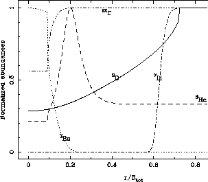
Figure 2: Normalized abundances in a ![]() non-standard model at the end
of the PMS. At that age (45 My) the convective core of the young Sun recedes and
the CZ is closed to its present day location. At LMR the solution is stable
even if
jumps of more than thirteen decades affect the diffusion coefficients. The
maxima respectively are:
non-standard model at the end
of the PMS. At that age (45 My) the convective core of the young Sun recedes and
the CZ is closed to its present day location. At LMR the solution is stable
even if
jumps of more than thirteen decades affect the diffusion coefficients. The
maxima respectively are:
![]() ,
, ![]() ,
, ![]() ,
,
![]() ,
, ![]()