In practice one may wish to repeat the algorithm for different shapes of the
target function ![]() and/or varying values of the
regularization parameter
and/or varying values of the
regularization parameter ![]() .
Changing the target functions requires re-computing steps
4, 5, 6 and 7. Changing
.
Changing the target functions requires re-computing steps
4, 5, 6 and 7. Changing ![]() requires re-computing steps 3, 5,
6 and 7. In Sect. 4 (click here) we will give a detailed analysis
of the number of operations used by the algorithm.
requires re-computing steps 3, 5,
6 and 7. In Sect. 4 (click here) we will give a detailed analysis
of the number of operations used by the algorithm.
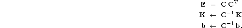
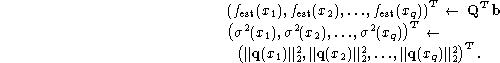
We can identify Eq. (9 (click here)) as an instance of the
well known equality constrained least squares problem (LSE); see
Lawson & Hanson (1974), Chap. 20. To realize this, let us
introduce the following quantities:
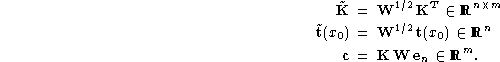
Using this notation we can write (9 (click here)) in the following
form:
![]()
These are in fact the normal equations for a constrained least squares
problem, for which we have the equivalent expression:
![]()
We can reformulate this as
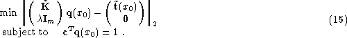
We now have an equality constrained least squares problem in
unit covariance form. Several methods have been developed for solving
problem LSE. Here we use the one described in Lawson & Hanson (1974), Chap. 20
and Golub & Van Loan (1989), Sect. 12.1.4.
The method has three stages:
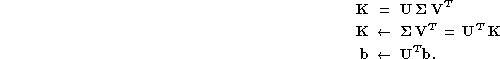
We can determine a parameterization of the set ![]() of vectors
in
of vectors
in ![]() that satisfy the constraint in Eq. (15 (click here)):
that satisfy the constraint in Eq. (15 (click here)):
![]()
To do this we compute an ![]() Householder transformation
Householder transformation
![]() (see Golub & Van Loan 1989, Sect. 5.2) such that
(see Golub & Van Loan 1989, Sect. 5.2) such that
![]()
In practice ![]() is not computed explicitly, but is represented in
the form
is not computed explicitly, but is represented in
the form ![]() . The columns of
. The columns of ![]() form a basis
for
form a basis
for ![]() and conceptually we can partition
and conceptually we can partition ![]() as
as
![]()
where ![]() .
It follows that
.
It follows that ![]() can be represented as
can be represented as
![]()
where ![]() is an arbitrary
(m-1)-vector (since all the columns of
is an arbitrary
(m-1)-vector (since all the columns of ![]() are orthogonal to
are orthogonal to ![]() ).
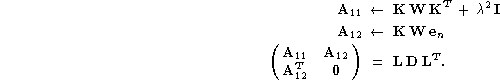
We can exploit this fact to transform problem LSE into the
following form, where we have inserted Eq. (16 (click here)) into
Eq. (15 (click here)) and collected terms:
).
We can exploit this fact to transform problem LSE into the
following form, where we have inserted Eq. (16 (click here)) into
Eq. (15 (click here)) and collected terms:
![]()
We now multiply from the left under the norm-sign with the orthogonal matrix
![]()
without changing the solution. Using the orthogonality of ![]() we
finally arrive at the reduced problem
we
finally arrive at the reduced problem
![]()
This is an ordinary unconstrained least squares problem. Having solved
this for ![]() we obtain the solution to the original constrained
problem as
we obtain the solution to the original constrained
problem as
![]()
We now describe an algorithm for solving (17 (click here)) which
is efficient when many values of ![]() are required.
Following Eldén (1977) we first bring
are required.
Following Eldén (1977) we first bring
![]() into bidiagonal form:
into bidiagonal form:
![]()
where
![]()
Here ![]() ,
, ![]() , and
, and ![]() is lower
bidiagonal. This is the most costly part of the computation, it
requires
is lower
bidiagonal. This is the most costly part of the computation, it
requires ![]() flops. The remaining part of the algorithm
only involves
flops. The remaining part of the algorithm
only involves ![]() , which means that the dimension of the problem is
effectively reduced from
, which means that the dimension of the problem is
effectively reduced from ![]() to
to ![]() . As in the SVD
transformation,
. As in the SVD
transformation, ![]() is not explicitly computed, but
is not explicitly computed, but ![]() is computed ``on the fly''. If
is computed ``on the fly''. If ![]() is required for
computing the discretized kernel
is required for
computing the discretized kernel ![]() , then the orthogonal
transformations that
, then the orthogonal
transformations that ![]() consists of are stored for later use. For
algorithmic details on bidiagonalization see, e.g.,
Golub & Van Loan (1989), pp. 236-238.
consists of are stored for later use. For
algorithmic details on bidiagonalization see, e.g.,
Golub & Van Loan (1989), pp. 236-238.
If we make the transformation of variables
![]()
then we easily see that (17 (click here)) is equivalent to
![]()
This least squares problem is now solved by determining a series of
2n-1 Givens rotations ![]() (see Golub & Van
Loan 1989,
Sect. 5.2) such that
(see Golub & Van
Loan 1989,
Sect. 5.2) such that
![]()
where ![]() is
is ![]() lower bidiagonal. The part of the
right-hand side denoted by ``
lower bidiagonal. The part of the
right-hand side denoted by ``![]() " consist of n non-zero elements
introduced along the way, but these are not computed in practice. We
illustrate this procedure on a small example with n=3. First a
rotation
" consist of n non-zero elements
introduced along the way, but these are not computed in practice. We
illustrate this procedure on a small example with n=3. First a
rotation ![]() applied to rows n and 2n annihilates the (2n,n)-element,
and a nonzero element is created in position (2n,n-1); then we annihilate
this element by a rotation
applied to rows n and 2n annihilates the (2n,n)-element,
and a nonzero element is created in position (2n,n-1); then we annihilate
this element by a rotation ![]() applied to rows 2n-1 and 2n:
applied to rows 2n-1 and 2n:
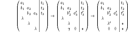
where
![]()
![]()
In the next step the same procedure is applied to the leading ![]() sub-matrix to annihilate the element in position
(2n-1,n-1), and so on. During the reduction we only need
to store the diagonals of
sub-matrix to annihilate the element in position
(2n-1,n-1), and so on. During the reduction we only need
to store the diagonals of ![]() in a pair of vectors, and the current
value of
in a pair of vectors, and the current
value of ![]() .
Now the solution
.
Now the solution ![]() can be computed as
can be computed as
![]()
For a large sparse or structured (e.g., Hankel or Toeplitz) matrix
![]() it is prohibitive to compute explicitly the full
bidiagonalization in Eq. (19 (click here)). Instead we would
prefer to keep
it is prohibitive to compute explicitly the full
bidiagonalization in Eq. (19 (click here)). Instead we would
prefer to keep ![]() in factored form
and use an iterative algorithm to solve the system
in (17 (click here)). An efficient and stable algorithm for doing
this, based on Lanczos bidiagonalization (Golub & Van
Loan 1989, Sect. 9.3.3), is the algorithm
LSQR, Paige & Saunders (1982a).
This algorithm only accesses the coefficient matrix
in factored form
and use an iterative algorithm to solve the system
in (17 (click here)). An efficient and stable algorithm for doing
this, based on Lanczos bidiagonalization (Golub & Van
Loan 1989, Sect. 9.3.3), is the algorithm
LSQR, Paige & Saunders (1982a).
This algorithm only accesses the coefficient matrix ![]() via
matrix-vector multiplications with
via
matrix-vector multiplications with ![]() and
and ![]() .
.
An even more efficient approach is to apply the LSQR algorithm
with ![]() and use the fact that the kth iterate
and use the fact that the kth iterate ![]() is a regularized solution. To be more specific, when we apply
LSQR to Eq. (17 (click here)) with
is a regularized solution. To be more specific, when we apply
LSQR to Eq. (17 (click here)) with ![]() , i.e.,
to
, i.e.,
to ![]()
then the iteration number k plays the role of the
regularization parameter; small k correspond to large ![]() , and
vice versa. The reason is that LSQR captures the spectral
components of the solution in order of increasing frequency, hence the
initial iterates are smoother than the iterations in later stages, and
as a consequence the initial iterates are more regularized.
, and
vice versa. The reason is that LSQR captures the spectral
components of the solution in order of increasing frequency, hence the
initial iterates are smoother than the iterations in later stages, and
as a consequence the initial iterates are more regularized.
The LSQR algorithm with ![]() is equivalent to Lanczos
bidiagonalization of
is equivalent to Lanczos
bidiagonalization of ![]() .
Specifically, after k steps, the Lanczos bidiagonalization algorithm
has produced three matrices
.
Specifically, after k steps, the Lanczos bidiagonalization algorithm
has produced three matrices ![]() ,
,
![]() , and
, and ![]() such that
such that
![]()
where both ![]() and
and ![]() have orthonormal columns,
and
have orthonormal columns,
and ![]() is bidiagonal.
Moreover, the first k columns of
is bidiagonal.
Moreover, the first k columns of ![]() , the first k-1 columns
of
, the first k-1 columns
of ![]() , and the leading
, and the leading ![]() sub-matrix of
sub-matrix of ![]() are identical to the corresponding quantities in the previous step of
the algorithm.
The kth iterate
are identical to the corresponding quantities in the previous step of
the algorithm.
The kth iterate ![]() is then computed as
is then computed as
![]()
where ![]() solves the problem
solves the problem
![]()
The key to the efficiency of LSQR lies in the way that ![]() is
updated to
is
updated to ![]() , while
, while ![]() and
and ![]() are
never stored; we refer to Paige & Saunders (1982a) for more details.
are
never stored; we refer to Paige & Saunders (1982a) for more details.
We emphasize the difference between the two bidiagonalization procedures.
The full bidiagonalization (19 (click here)) is explicitly computed once, and
it is independent of the regularization parameter; ![]() enters
when solving the augmented bidiagonal system in Eq. (22 (click here)).
The Lanczos bidiagonalization appears implicitly in computing the
LSQR iterates
enters
when solving the augmented bidiagonal system in Eq. (22 (click here)).
The Lanczos bidiagonalization appears implicitly in computing the
LSQR iterates ![]() , and the sequence of iterates
, and the sequence of iterates
![]() corresponds to sweeping through
a range of regularization parameters.
corresponds to sweeping through
a range of regularization parameters.
To compute the solution to the original problem in (15 (click here)) it is
necessary to transform the solution ![]() or
or ![]() to the original variable
to the original variable ![]() .
Below
.
Below ![]() and
and ![]() denote either
denote either
![]() and
and ![]() from Sect. 2.2.2 (click here) or
from Sect. 2.2.2 (click here) or
![]() and
and ![]() from Sect. 2.2.3 (click here).
Inserting Eq. (18 (click here)) and
(21 (click here)) in Eq. (2 (click here)) we get
from Sect. 2.2.3 (click here).
Inserting Eq. (18 (click here)) and
(21 (click here)) in Eq. (2 (click here)) we get
Similarly, if we insert Eqs. (18 (click here)),
(19 (click here)) and (21 (click here)) in Eq.
(10 (click here)) and use the definition of ![]() then we get
then we get
Finally, due to the orthogonality of ![]() and
and ![]() the variance of the error in
the variance of the error in ![]() due to the noise takes the form
due to the noise takes the form
Consider first full bidiagonalization from Sect. 2.2.2 (click here).
We notice that ![]() is the only quantity in the
above expressions that depends on the regularization parameter
is the only quantity in the
above expressions that depends on the regularization parameter ![]() and the target function
and the target function ![]() .
Therefore
.
Therefore ![]() and
and ![]() only need to be
computed once (in fact, they are already computed in earlier stages of
the algorithm).
This means that re-computing the solution
only need to be
computed once (in fact, they are already computed in earlier stages of
the algorithm).
This means that re-computing the solution ![]() when changing
when changing ![]() or
or
![]() is very cheap.
This is a great improvement
compared with the Lagrange-multiplier method from Sect. 2.1 (click here),
where a matrix factorization must re-computed each time.
is very cheap.
This is a great improvement
compared with the Lagrange-multiplier method from Sect. 2.1 (click here),
where a matrix factorization must re-computed each time.
Although we do not explicitly compute ![]() , it is still quite
inexpensive to compute the discretized averaging kernels
, it is still quite
inexpensive to compute the discretized averaging kernels ![]() for the different solutions.
Again, one of the terms, namely
for the different solutions.
Again, one of the terms, namely ![]() , is already computed
in earlier steps of the algorithm and the term
, is already computed
in earlier steps of the algorithm and the term ![]() requires only approximately
requires only approximately ![]() flops.
flops.
Consider next the case from Sect. 2.2.3 (click here) where we use
Lanczos bidiagonalization. Again, only ![]() depends on
the target function
depends on
the target function ![]() , but now both
, but now both ![]() and
and ![]() depend on the regularization parameter, i.e., the iteration number k.
Moreover, they both appear only implicitly in the algorithm, while it
is the iteration vector
depend on the regularization parameter, i.e., the iteration number k.
Moreover, they both appear only implicitly in the algorithm, while it
is the iteration vector ![]() that is explicitly computed.
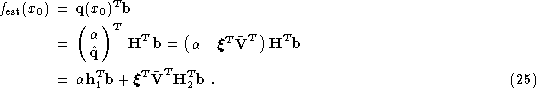
It is now more efficient to use the formulation
that is explicitly computed.
It is now more efficient to use the formulation
![]() to compute
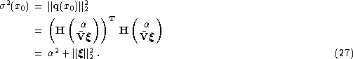
the estimated solution, and the variance of the error in
to compute
the estimated solution, and the variance of the error in ![]() is given by
is given by
![]() .
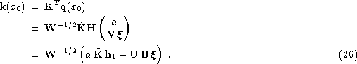
Similarly, the discretized averaging kernel should be computed by
means of
.
Similarly, the discretized averaging kernel should be computed by
means of ![]() .
.
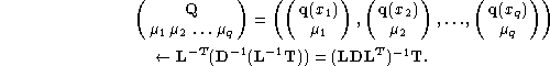
Our new algorithms, based on bidiagonalization, are summarized
below. They describe the general case where ![]() is computed at
points
is computed at
points ![]() . The matrix
. The matrix ![]() below is again the matrix
whose columns contain ``samples'' of the q target function:
below is again the matrix
whose columns contain ``samples'' of the q target function:
![]() ,
, ![]() ,
,
![]() .
.