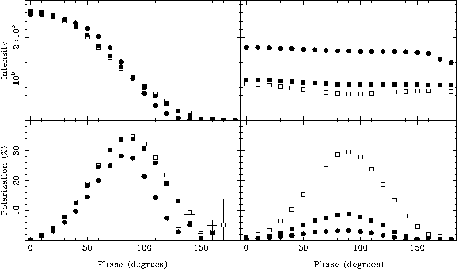
Figure 11: The phase dependence of scattering models. The left-hand panel
shows results for a simple `reflection' model (Sect. 7.1 (click here)) with
![]() (open squares),
(open squares), ![]() (filled
squares), and
(filled
squares), and ![]() (filled circles); the right-hand panel
shows results for the reference model (Sect. 7.2 (click here); filled
circles) and for models with moderate and extensive ionized zones
(Sect. 6.2 (click here); filled and open squares, respectively). In each
case the top panel shows
the line intensity and the bottom panel shows the line polarization.
Error bars are one sigma
(filled circles); the right-hand panel
shows results for the reference model (Sect. 7.2 (click here); filled
circles) and for models with moderate and extensive ionized zones
(Sect. 6.2 (click here); filled and open squares, respectively). In each
case the top panel shows
the line intensity and the bottom panel shows the line polarization.
Error bars are one sigma
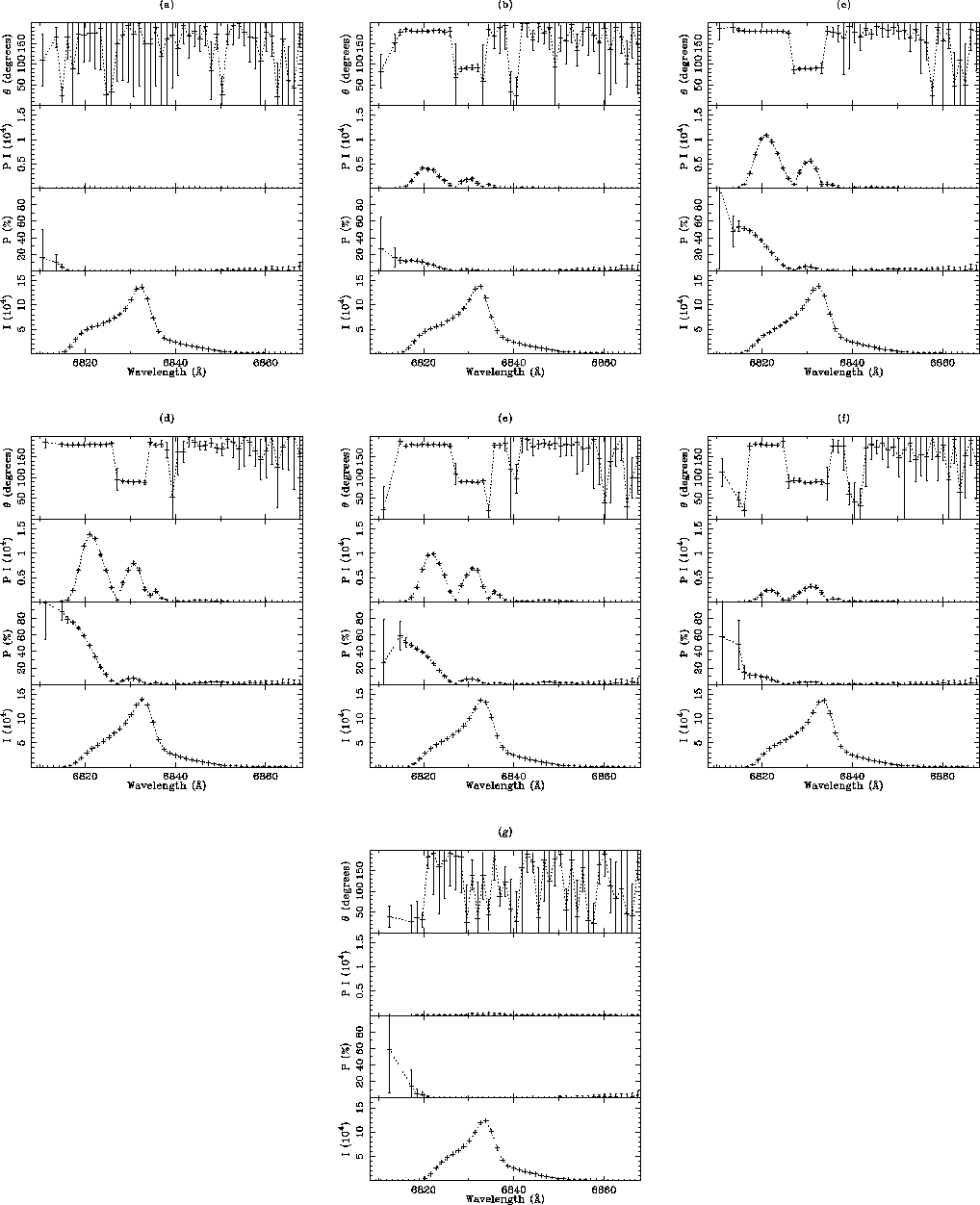
Figure 12: Raman-line polarization spectra of the reference model with viewing
angles of ![]() -
-![]() at steps of 30
at steps of 30![]() a-g)
a-g)
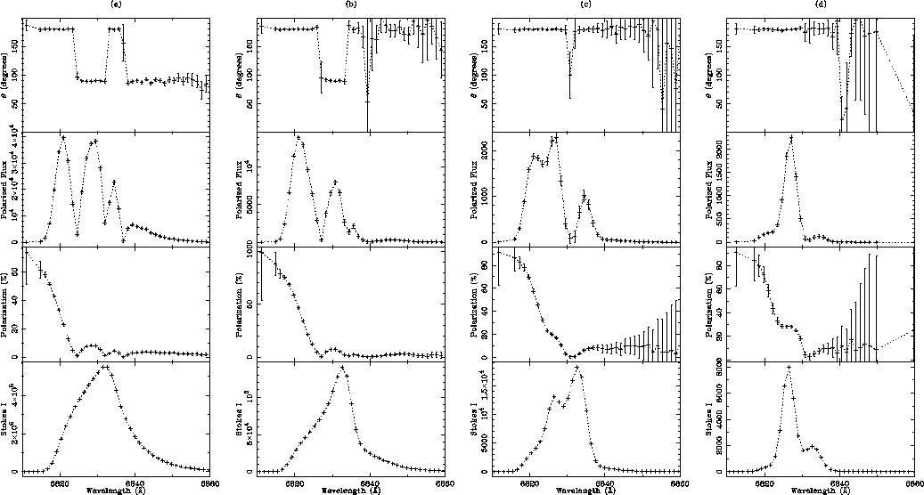
Figure 13: Raman-line polarization spectra for models viewed at
quadrature, with mass-loss rates of a) ![]() , b)
, b) ![]() , c)
, c) ![]() and
d)
and
d) ![]() (cf. Sect. 8 (click here)). Other parameters are those of the
reference model
(cf. Sect. 8 (click here)). Other parameters are those of the
reference model
Figure 14: Raman-line polarization spectra for models with wind
velocities of a) ![]() =10 kms
=10 kms![]() , b)
, b)
![]() =50 kms
=50 kms![]() and
and ![]() =100 kms
=100 kms![]() ,
plotted in Raman `parent' velocity space (cf. Sect. 9.1 (click here)). The
mass-loss rate for models a) and c) were
adjusted so that
,
plotted in Raman `parent' velocity space (cf. Sect. 9.1 (click here)). The
mass-loss rate for models a) and c) were
adjusted so that ![]() was equal to that of model b).
Other parameters are those of the reference model
was equal to that of model b).
Other parameters are those of the reference model
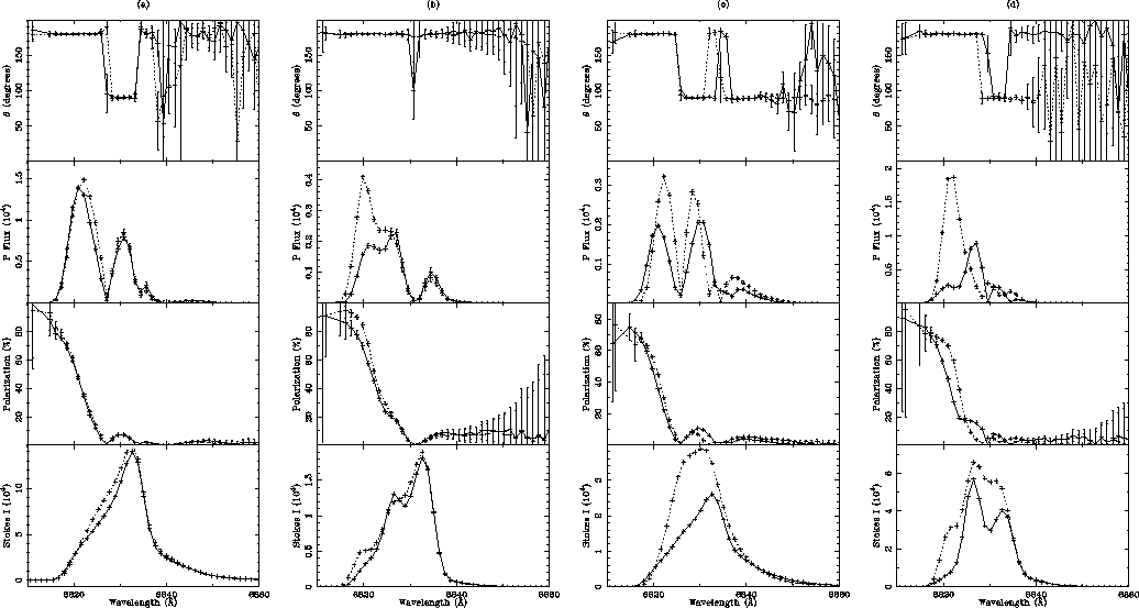
Figure 15: Raman-line polarization spectra for models computed with a
constant-velocity
wind (solid line) and with a velocity law
![]() (dotted line; cf. Sect. 9.2 (click here)). The parameters are those of
the reference model (
(dotted line; cf. Sect. 9.2 (click here)). The parameters are those of
the reference model (![]() km s
km s![]() )
except a)
)
except a) ![]() ,
, ![]() b)
b)
![]() ,
, ![]() c)
c) ![]() ,
, ![]() and d)
and d) ![]() ,
, ![]()
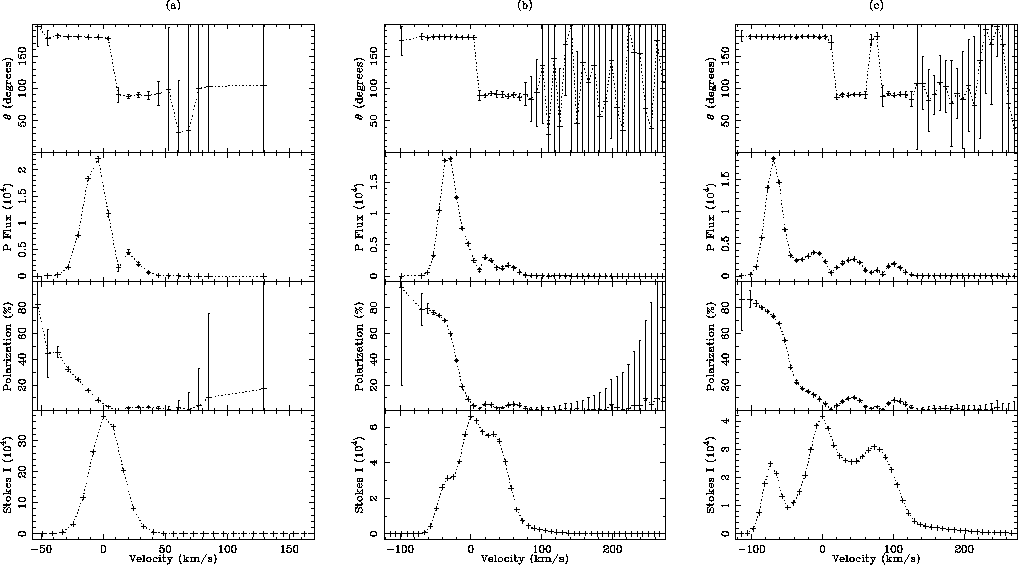
Figure 16: Raman-line polarization spectra for models with a velocity law
![]() ,
, ![]() , and
, and ![]() (cf. Sect. 9.2 (click here)).
Other parameters are those of the reference model, except
a)
(cf. Sect. 9.2 (click here)).
Other parameters are those of the reference model, except
a)
![]() =10 kms
=10 kms![]() , b)
, b) ![]() =50 kms
=50 kms![]() , and
c)
, and
c) ![]() =100 kms
=100 kms![]()
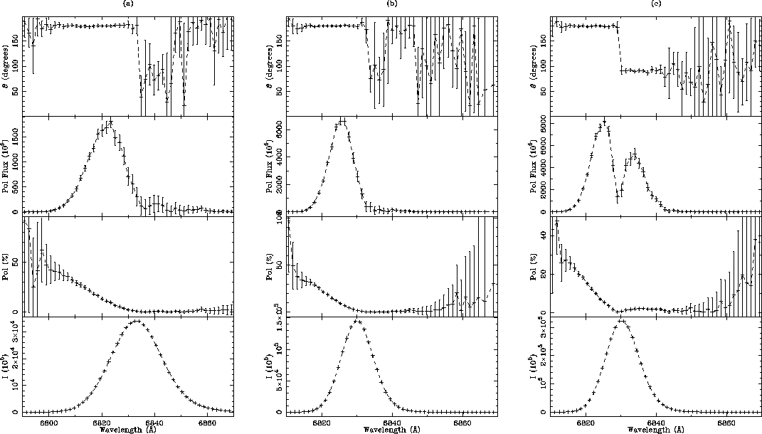
Figure 17: Raman-line models for ![]() /parent OVI
/parent OVI ![]() 1032 Å
FWHM/red-giant wind velocity combinations of a) [-6.0/100/50],
b) [-6.3/50/20] and c) [-6.0/50/20], observed at quadrature (cf.
Sect. 9.3 (click here))
1032 Å
FWHM/red-giant wind velocity combinations of a) [-6.0/100/50],
b) [-6.3/50/20] and c) [-6.0/50/20], observed at quadrature (cf.
Sect. 9.3 (click here))
Two test models have been run, with ![]() =10 kms
=10 kms![]() and
and
![]() =100 kms
=100 kms![]() , to check the response
of the models to changes in wind velocity. The mass-loss rates
were adjusted such that
, to check the response
of the models to changes in wind velocity. The mass-loss rates
were adjusted such that ![]() - and hence
- and hence ![]() -
was constant, so as to isolate velocity effects from density effects.
In order to examine the velocity structure of the lines the model
profiles, presented in (Fig. 14 (click here)), have been converted to `Raman
parent'
velocity space. The wavelength of the Raman parent photon
-
was constant, so as to isolate velocity effects from density effects.
In order to examine the velocity structure of the lines the model
profiles, presented in (Fig. 14 (click here)), have been converted to `Raman
parent'
velocity space. The wavelength of the Raman parent photon ![]() is given by
is given by
![]()
where ![]() is the Raman-scattered wavelength and
is the Raman-scattered wavelength and ![]() is the wavelength of Ly
is the wavelength of Ly![]() . The Raman parent
wavelength may thus be converted to velocity space by using the rest
wavelength of the Raman parent line.
. The Raman parent
wavelength may thus be converted to velocity space by using the rest
wavelength of the Raman parent line.
The ![]() =10 kms
=10 kms![]() model gives an almost symmetrical
profile that is redshifted by about 10 kms
model gives an almost symmetrical
profile that is redshifted by about 10 kms![]() . There is a
single peak in the polarized flux spectrum that is blueshifted by
approximately 10 kms
. There is a
single peak in the polarized flux spectrum that is blueshifted by
approximately 10 kms![]() (the reference model has a much broader
intensity profile that peaks at approximately 40 kms
(the reference model has a much broader
intensity profile that peaks at approximately 40 kms![]() , and
the polarized-flux peaks occur at -40 kms
, and
the polarized-flux peaks occur at -40 kms![]() and
30 kms
and
30 kms![]() ). The
). The ![]() =100 kms
=100 kms![]() model has a
highly asymmetric intensity profile that has a redshifted peak at
approximately 90 kms
model has a
highly asymmetric intensity profile that has a redshifted peak at
approximately 90 kms![]() . The polarized flux spectrum shows
three peaks. The blueshifted peak lies at -80 kms
. The polarized flux spectrum shows
three peaks. The blueshifted peak lies at -80 kms![]() , the
middle peak at 60 kms
, the
middle peak at 60 kms![]() and the redmost peak lies at about
110 kms
and the redmost peak lies at about
110 kms![]() .
.
These results confirm intuitive expectations that the peak-to-peak
separations of the polarization profiles should be a function of the
local velocity field, and demonstrate that, provided sufficient wind
density exists to ensure that scattering occurs over a reasonable
volume, the separations of the polarization peaks provide a useful guide
to the velocity gradients in the outflow. Because of projection
effects, those separations will always be less than the true velocity
contrasts, and thus will provide a conservative lower limit if used to
estimate wind speeds. The characteristic peak separations of the
observations reported in Paper I is ![]() 50 kms
50 kms![]() , suggesting
that the outflow velocities close to the binary system are rather larger
than the canonical 10 kms
, suggesting
that the outflow velocities close to the binary system are rather larger
than the canonical 10 kms![]() .
.
The reference model employs a constant-velocity wind. Clearly this is
an
unrealistic assumption and, since the Raman-line velocity structure is
most simply explained in terms of scattering in a moving medium, it is
of particular interest to examine the effects of different velocities
and acceleration laws on the Raman lines. Several models were computed
in order to investigate the effects of an accelerating wind on the Raman
lines. A velocity law of the form
![]()
was adopted, solely because, in common with a constant-velocity flow, it
has a computationally cheap analytical solution for the mass-column
integral over any path in the wind. This velocity law is slightly
steeper than those considered by Vogel (1991) when interpreting
observations of a Rayleigh-scattering `eclipse' in EG And. His
empirical velocity law has a low, constant velocity out to a few stellar
radii, where the wind rapidly accelerates to its terminal speed.
Four models were run, using ![]() and
and ![]() for
binary separations of
for
binary separations of ![]() and
and ![]() (Fig. 15 (click here)), together with constant-velocity models for
comparison. Model (a) shows only minor differences between the
Raman line produced by the comparison (reference) model and that
produced by the accelerating-wind law. The accelerating-wind models
show mild intensity and polarized-flux increases on the blue side of the
profile, while the red wings are almost identical.
Model (b), with
(Fig. 15 (click here)), together with constant-velocity models for
comparison. Model (a) shows only minor differences between the
Raman line produced by the comparison (reference) model and that
produced by the accelerating-wind law. The accelerating-wind models
show mild intensity and polarized-flux increases on the blue side of the
profile, while the red wings are almost identical.
Model (b), with ![]() , shows marked differences in both the
intensity and polarized-flux profiles between the accelerating and
constant-velocity models. The major changes occur in the blue side of
the profile, with the accelerating-wind model displaying a much larger
polarized flux in the bluemost peak. The red side of the profile is
again almost unchanged, both in total flux and polarized flux.
, shows marked differences in both the
intensity and polarized-flux profiles between the accelerating and
constant-velocity models. The major changes occur in the blue side of
the profile, with the accelerating-wind model displaying a much larger
polarized flux in the bluemost peak. The red side of the profile is
again almost unchanged, both in total flux and polarized flux.
Model (c), with a mass-loss rate of ![]() and
and ![]() , shows further differences between the two wind structures. The
intensity profile of the accelerating-wind model is much stronger, and,
although the line polarization is less than the constant-velocity model
at the line centre, the polarized flux is greater.
The final model, (d), with a lower mass-loss rate and
with a small binary separation, gives very different profiles for an
accelerating wind. The intensity profile is stronger, with a central
peak and red- and blue-shifted shoulders. The polarized-flux profile
shows a single strong peak which is blue-shifted with respect to the
intensity maximum.
, shows further differences between the two wind structures. The
intensity profile of the accelerating-wind model is much stronger, and,
although the line polarization is less than the constant-velocity model
at the line centre, the polarized flux is greater.
The final model, (d), with a lower mass-loss rate and
with a small binary separation, gives very different profiles for an
accelerating wind. The intensity profile is stronger, with a central
peak and red- and blue-shifted shoulders. The polarized-flux profile
shows a single strong peak which is blue-shifted with respect to the
intensity maximum.
These models demonstrate that the velocity structure of the cool wind can have a strong effect on the Raman lines, both in terms of the intensity profile and the polarization structure. The smallest differences between the constant-velocity wind and the accelerating-wind models occur at the larger binary separations, particularly for winds with high mass-loss rates, because the line formation in the accelerating model is then occurring in regions where the wind is close to its terminal velocity, with little scattering occurring in the steeply accelerating region of the wind.
When significant changes do occur between the constant-velocity and accelerating models, the blue wing shows the most sensitive response. This is because the inter-component region is the scattering volume most affected by the choice of velocity law; the slower the velocity law, the denser the wind in (especially) this region, and the lower the velocity of the scatterers. Thus model (b) shows that the velocity law can be important even in models with lower mass-loss rates and wide binary separations. Clearly, though, the velocity structure becomes most important when the binary separation is small, when the line formation is occurring in a region of the wind with large radial velocity gradients. Model (c) shows that the Raman-line intensity is stronger in the accelerating-wind model, mainly because the wind density is much higher at smaller separations than in the constant-velocity model.
Further accelerating-wind models were computed for a small binary
separation (![]() ) and low mass-loss rate (
) and low mass-loss rate (![]() ),
and a range of terminal velocities (Fig. 16 (click here)). These
models demonstrate the complex structures that can be obtained when the
lines are formed in the accelerating region of the wind, when photons
are being scattered in the approaching and receding parts of the wind,
and in the photosphere. Model 16 (click here)(b), in particular,
resembles many of the observations presented in Paper I in terms of its
PA structure (cf. Fig. 6 (click here)). The intensity
profile shows a strong central peak with blue- and red-shifted
shoulders, while the polarized-flux spectrum shows a strong blue-shifted
peak and two smaller red-shifted ones that are barely resolved. The
blue- and red-shifted peaks are perpendicularly polarized. This model
has a low mass-loss rate and a small scattering volume, but because the
binary separation is small a PA flip is observed, unlike the
),
and a range of terminal velocities (Fig. 16 (click here)). These
models demonstrate the complex structures that can be obtained when the
lines are formed in the accelerating region of the wind, when photons
are being scattered in the approaching and receding parts of the wind,
and in the photosphere. Model 16 (click here)(b), in particular,
resembles many of the observations presented in Paper I in terms of its
PA structure (cf. Fig. 6 (click here)). The intensity
profile shows a strong central peak with blue- and red-shifted
shoulders, while the polarized-flux spectrum shows a strong blue-shifted
peak and two smaller red-shifted ones that are barely resolved. The
blue- and red-shifted peaks are perpendicularly polarized. This model
has a low mass-loss rate and a small scattering volume, but because the
binary separation is small a PA flip is observed, unlike the ![]() model.
model.
The widths of the Raman lines are primarily determined by both the
velocity field of the red-giant wind and the intrinsic width of the
scattered OVI lines. As noted in Sect. 4.1 (click here),
observations of NV suggest line widths (FWHM) typically in
the range 50-70 km![]() ; moreover, the line widths increase
with increasing ionization potential. We have therefore investigated
the effects of adopting broader OVI lines than those of the
reference model (FWHM=20 km
; moreover, the line widths increase
with increasing ionization potential. We have therefore investigated
the effects of adopting broader OVI lines than those of the
reference model (FWHM=20 km![]() ).
).
Figure 17 (click here)a shows the results of a calculation with
FWHM=100 kms![]() , and the reference-model red-giant wind
velocity. The intensity profile (and, to a lesser extent, the
polarized-flux spectrum) is completely unstructured, and has a
FWHM of
, and the reference-model red-giant wind
velocity. The intensity profile (and, to a lesser extent, the
polarized-flux spectrum) is completely unstructured, and has a
FWHM of ![]() 1000 kms
1000 kms![]() . (The `resolution boosting' of the
Raman scattering, by a factor
. (The `resolution boosting' of the
Raman scattering, by a factor ![]() (Raman)/
(Raman)/![]() (Parent),
means that the input profile would be broadened to
(Parent),
means that the input profile would be broadened to
![]() 670 kms
670 kms![]() even in a static scattering medium.) This is
in contrast to the observed lines, which are nearly always highly
structured when observed with adequate resolution (Fig. 6 (click here);
Paper I), and which are rarely as broad as the model shown in
Fig. 17 (click here).
even in a static scattering medium.) This is
in contrast to the observed lines, which are nearly always highly
structured when observed with adequate resolution (Fig. 6 (click here);
Paper I), and which are rarely as broad as the model shown in
Fig. 17 (click here).
One might ask if the line width and lack of structure in the intensity
profile results from smearing due to the rather large red-giant wind
velocity used in the reference model. To address this question we
show in Fig. 17 (click here)b a model calculated with `canonical'
parameters: an OVI line-width of 50 kms![]() and a
wind velocity of 20 kms
and a
wind velocity of 20 kms![]() , with
, with ![]() held at
the reference-model value. The intensity profile remains
symmetrical and unstructured, with a single polarization peak
which primarily arises from scattering close to the line of centres
between the stars.
held at
the reference-model value. The intensity profile remains
symmetrical and unstructured, with a single polarization peak
which primarily arises from scattering close to the line of centres
between the stars.
The crucial point of these models is that the velocity width of the OVI line exceeds the asymptotic velocity of the wind. Hence, the polarization structure can no longer be simply attributed to wind broadening and the effects of spectral smearing must be considered. Figure 17 (click here)a, for example, has a much reduced red-shifted polarized flux peak. This is because although the mass-loss rate is the same as the reference model (i.e. the number of scatterings above and below the source is the same), the broad OVI line means that some photons scattered between the source and the red-giant (polarized perpendicularly to the red-shifted peak) have the same wavelength as photons scattered above and below the source, leading to partial cancellation of Stokes Q, particularly in the red wing.
To produce a significantly structured polarization spectrum requires an increase in mass-loss rate (i.e., in scattering optical depth). Figure 17 (click here)c shows a model calculated for the reference-model mass-loss rate. The intensity profile is still unstructured, but the extra scattering optical depth is sufficient to introduce an additional redshifted feature, which, since it is polarized orthogonally to the main peak, clearly originates `above/below' the OVI source.
These results show that to provide significant structure in the Raman
lines (as is nearly always observed) within the framework of the adopted
geometry, it is necessary to have a reasonably small OVI line
width. The models discussed here therefore provide some justification
for the relatively low FWHM adopted in the reference model, and suggest
that the scattered component of the OVI lines may be no more
than a few tens of km![]() broad.
broad.