6 The XMM-OM multicolour space and quasars

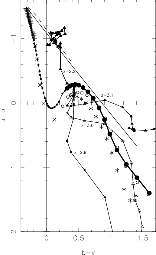
In the present section, we investigate the ability of the XMM-OM photometric system to segregate quasars from stars on the basis of their colours in the multicolour space definable from the set of the different filters used. Therefore, we integrated both the stellar spectra discussed in Sect. 2.3 and the average quasar spectra discussed in Sect. 2.4. The latter ones have been considered at redshifts from 0.0 to 4.4 by steps of 0.1. We start our analysis with the XMM-OM version of the classical (U-B) vs. (B-V) colour diagram.

6.1 The basic (u-b) vs. (b-v) diagram

The (U-B) vs. (B-V) colour diagram is probably one of the most widely used in astronomy. Therefore, Fig. 7 presents the XMM-OM version ((u-b) vs. (b-v)) of this diagram. Fortunately, no huge difference appears between the two versions and the XMM-OM colour diagram retains most of the properties of its classical counterpart.

Figure 7: The (u-b) vs. (b-v) colour diagram. The halo main sequence stars are represented by filled circles; the part of the sequence populated in our Galaxy is in bold character. The halo giants are represented by open circles whereas the cool end of the disk main sequence is described by asterisks. The crosses stand for the HB BA stars whereas the plus signs deal with the sd OB stars. The continuous line represents the black body locus and the dashed line the positions of the degenerate stars as derived from Koester's models. Model A average quasar spectrum has its redshift track punctuated with filled triangles every 0.1 in redshift whereas model B is marked out by open triangles and model C by filled squares. The highest plotted redshifts are 4.1, 3.7 and 3.1 for the quasars of models A, B and C respectively

The locus of the theoretical halo main sequence stars is given (filled circles). The classical potential-well shape of the curve outlining the effect of the Balmer continuum is clearly visible. The part below the turn-off represents the stars that are still on the main sequence in the halo of our Galaxy; it is represented by a bold line. This bold line is the locus of the majority of the field stars which are the objects against which we have to perform the basic discrimination when looking for quasars. The locus of cool giants is also given (open circles) and is very similar to the previously discussed one. On the other hand, the disk main sequence (spectral types FGKM), which could also provide some confusion, is visible below the halo main sequence (asterisks). The HB stars (crosses) have colours very similar to the hot part (astronomically non populated) of the halo main sequence. This is also true for the sdOB stars (plus signs). These objects are classical contaminants of the samples of quasar candidates selected on the basis of the U/B excess. Another contaminant are the degenerate stars. The black body line is also given in Fig. 7 and the Koester's models whose spectrum we integrated fall close to this line. Figure 7 also exhibits the track of our average quasars as a function of redshift. For redshifts z $\leq$ 2.1, the average quasars are wandering around u-b = -1.0 and b-v = 0.15. This is 0.2 magnitude bluer in u-b than in the case of the standard system (see e.g. Fig. 6 of Cristiani & Vio 1990 and Fig. 9 of Moreau & Reboul 1995). This ability to better detect the bluer objects is essentially due to the comparatively high transmission of the u filter below 3200 Å (see Fig. 1b and Sect. 2.1).

The wandering around the mean place is essentially due to the various emission lines entering and going out of the different filters but also partly to the particular shapes of the top of the transmission curves. The region around this mean place is also where one can find degenerate stars (with typical $T_{\rm eff} \sim 15000$ K) and the presently investigated colour combination is not useful in discriminating between both kind of objects. At z = 2.2, the quasars have left their low-redshift location to move almost parallel to the (u-b) axis. This is due to the fact that the Ly$\alpha$ emission line is leaving the u filter to enter the bone and is progressively replaced by the Ly$\alpha$ forest. This occurs 0.07 earlier in redshift than in the Johnson standard system.

The tracks of the average quasars are also given for higher redshifts. It should however be clearly stated that for redshifts $z~\geq~2.9$, both the u and the b filters are mainly sampling the Ly$\alpha$ forest and the related quasar location in the bidimensional (2D) colour diagram is highly model dependent. It is interesting to notice that the model B spectra tend to follow the stellar locus whereas model C quasars stay bluer in b-v. In any case, the discrimination is essentially possible for low-redshift ( $z~\leq~2.2$) quasars and for high-redshift weakly or strongly absorbed objects.

Figure 8 gives the distance (in this two-dimensional space) between the model A quasar and the stellar locus as a function of redshift (by steps of 0.1, filled circles). The stellar locus adopted here is the whole halo main sequence. Except for degenerate stars, this locus can be considered as representative of most of the other potential contaminants.

Figure 8 clearly demonstrates the ability to discriminate between non-degenerate stars and quasars with redshifts $z\leq 2.2$. In the range $z \in[2.2, \sim 3.]$ (or more), quasars have ubv colours very similar to stars and the discrimination power will only improve through the use of additional filters. The apparent improvement for redshifts in the range $z \in[3.3,3.6]$ is not present for model B quasars: this pinpoints the model dependent character of this particular result.

At z>3.8, all three filters are essentially in the Ly$\alpha$ forest and the increase in distance is indicative of a potential discrimination but the latter is bound to be highly dependent on the particular realization of the distribution of the Ly$\alpha$absorbers both in redshift and in density. The completeness of the related sample will be hard to ascertain.

Figure 8: The reduced distance between the average model A quasar and the stellar locus as a function of redshift, by steps of 0.1. The first curve (circles) represents the two-dimensional distance in the 2D (u-b) vs. (b-v) colour diagram as given in Fig. 7. The second curve (triangles) represents $\sqrt {2} / \sqrt {3}$ times the three-dimensional distance in the 3D (uvw1-u) vs. (u-b) vs. (b-v) colour diagram. The third curve (stars) gives $\sqrt {2} / \sqrt {4}$ times the four-dimensional distance in the 4D (uvw2-uvw1) vs. (uvw1-u) vs. (u-b) vs. (b-v) colour diagram

6.2 Adding uvw1

Our simulations concerning the uvw1 filter clearly indicate that this filter is roughly as sensitive to the Balmer continuum (not to confuse with the Balmer jump) as the u filter. The (uvw1-b) colour index of stars has a behaviour very similar to the (u-b) one and the locus of stars in a (uvw1-b) vs. (b-v) diagram is very reminiscent of Fig. 7. The (uvw1-u) colour index is much less sensitive to the Balmer continuum. It is interesting to notice that in a 2D (uvw1-u) vs. (uvw1-v) colour diagram, the quasars with $z\leq 1.5$ are perfectly superimposed on the locus of stars. Therefore, this combination is not interesting for low-redshift quasars but quasars with redshifts between 1.6 and 2.1 are moving away from the stellar locus in the same diagram. This is essentially due to the Ly$\alpha$ emission line leaving uvw1 for the u filter and to the Ly$\alpha$forest becoming dominant in uvw1. Nevertheless, full exploitation of this phenomenon requires observations in the b filter. This is particularly striking in the (uvw1-u) vs. (u-b) colour diagram (not shown here).

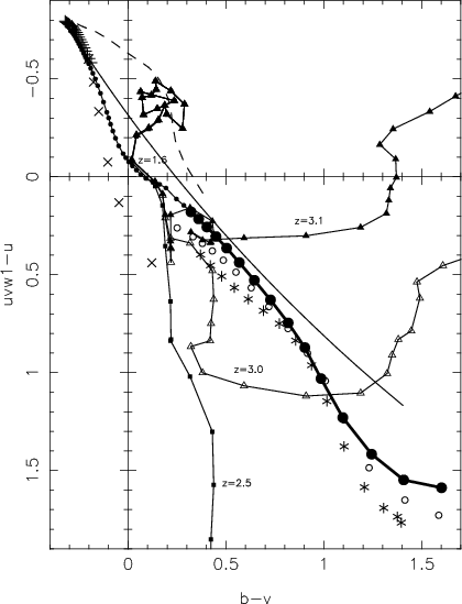Figure 9: The (uvw1-u) vs. (b-v) colour diagram. The symbols have the same meaning as those used for Fig. 7. The highest plotted redshifts are 4.1, 3.9 and 2.6 for the quasars of models A, B and C respectively

Figure 9 gives the 2D (uvw1-u) vs. (b-v) colour diagram. At redshifts $z\leq 1.5$, quasars are wandering around uvw1-u = -0.4 and b-v = 0.15. This is slightly aside the non-degenerate stellar locus and the uvw1 filter contributes, although weakly, to the star-quasar separation. For redshifts $1.6 \leq z \leq 3.0$, the average quasar joins the stellar locus in this 2D diagram of Fig. 9 but it is known to deviate from the stellar locus in the (uvw1-u) vs. (uvw1-v) colour diagram for $1.6 \leq z \leq 2.1$. In Fig. 8 is also given the distance between the quasar and the stellar locus in the three-dimensional space (uvw1-u) vs. (u-b) vs. (b-v). Increasing the number of dimensions of the space always brings an increase of the distance between objects, although the effect is purely geometrical. To test whether or not the added filter brings a strategical contribution due to its location in the wavelength domain, one has to compare the distances reduced to the lower dimension space. Therefore, in Fig. 8, we compare the two-dimensional true distance (in (u-b) vs. (b-v)) to the reduced 3D distance which is the three-dimensional true distance (in (uvw1-u) vs. (u-b) vs. (b-v)) multiplied by a $\sqrt {2} / \sqrt {3}$ factor.

From Fig. 8, it is absolutely clear that the main contribution of the use of uvw1 to the discriminating power of the XMM-OM photometry is essentially located at the redshift range 1.6 to 2.1. It is also interesting to notice that low-redshift quasars are wandering in Fig. 9 slightly aside the black body line. However, the degenerate stars do not follow the black body locus but, rather, are again mixed with low-redshift quasars (a typical effective temperature for a white dwarf in the middle of the low-redshift quasar locus is 12 000 K). This suggests that the discrimination between degenerate stars and quasars is bound to remain poor. Beyond z = 3.0, the model A quasars seem to remain out of the stellar locus, and the model C quasars stay bluer in b-v. This again depends on the particular behaviour of the Ly$\alpha$ absorbers in the line of sight of the observed quasar.

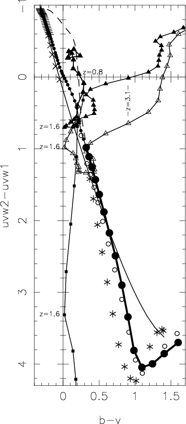Figure 10: The (uvw2-uvw1) vs. (b-v) colour diagram. The symbols have the same meaning as those used for Fig. 7. The highest plotted redshifts are 4.1, 3.9 and 1.8 for the quasars of models A, B and C respectively

6.3 Adding uvw2

Filter uvw2 could also be used to build-up colour diagrams. However, it should be kept in mind that the XMM-OM is not very sensitive in this passband and the precision of the measurement in uvw2 could be markedly worse than in any of the other filters. The use of filter uvw2 is illustrated in Fig. 10 where the 2D (uvw2-uvw1) vs. (b-v) colour diagram is given. Similarly to the previous case, low-redshift ($z\leq 0.6$) quasars are wandering at (uvw2-uvw1) = -0.3 and, of course, (b-v) = 0.15. This is slightly out of the stellar locus. However, at $z\sim 0.7$, the average quasars progressively become redder in (uvw2-uvw1) due as usual to the Ly$\alpha$ emission line going from the first filter to the second. The present colour index is expected to be discriminant when the Ly$\alpha$ line is located in the uvw1 filter, i.e. roughly for redshifts between 0.8 and 1.6. This is easily seen in the (uvw2-uvw1) vs. (uvw1-u) colour diagram as well as in the (uvw2-uvw1) vs. (uvw1-b) one; this pinpoints the importance of the joint use of the u filter (or perhaps the b one) along with the pair uvw2, uvw1. Figure 8 exhibits the reduced ( $\sqrt{2} / \sqrt{4} = 1 / \sqrt{2}$) four-dimensional distance in the 4D (uvw2-uvw1) vs. (uvw1-u) vs. (u-b) vs. (b-v) colour space. It is clear that the contribution of the uvw2 filter contrasting with the uvw1 one is increasing the discrimination power in the redshift range 0.8 to 1.6. This effect could help in generating quasar samples that are more homogeneous in redshift since the use of the new filters alleviates the well-known bias of U/B selected quasar candidates due to the presence of a strong C  IV line in the B filter (at $z \sim 1.6 - 1.7$). From Fig. 10, it is again clear that the degenerate stars do not follow the black body line and that they still remain a strong contaminant of the samples of quasars (particularly around $T_{\rm eff} \sim 13000$ K).

6.4 General considerations

From Fig. 8, one can conclude that the XMM-OM filter set is good at discriminating between non-degenerate stars and quasars at low redshifts ( $z~\leq~2.2$). This is particularly true in the range 0.8 to 2.1 where the use of the uvw1 and uvw2 filters allows a significantly better discrimination that is even able to wash out the decrease in efficiency around $z~\sim~1.6 - 1.7$ sometimes exhibited by traditional (U-B) vs. (B-V) surveys. For very low redshifts (z < 0.8), the advantage of this photometric system is less marked. However, one should not forget that Fig. 8 gives the reduced distance. Indeed, the minimum true distance between the quasar and the stellar locus is, in the 4D space of Sect. 6.3, somewhat larger than 0.35 magnitudes (occuring at z=0.5); this already implies a real possibility of segregation. For redshifts between 2.3 and 3.5, the selection is essentially inefficient, as for ground-based surveys neglecting the use of the R and I filters (for example). It is beneficial to recall that XMM-OM was originally designed with a red optical path that has been abandoned in the meantime. Beyond z = 3.5, the average quasar is usually off the stellar locus but this corresponds to the presence of the Ly$\alpha$ forest in most of the filters and is thus again highly dependent on the particular realization of the Ly$\alpha$ absorption (density and actual locations of the strong Ly$\alpha$ absorbers on the line of sight). In addition, the flux below Ly$\alpha$ is comparatively much lower implying a far less precise photometry. Generally, it is clear that the XMM-OM filter set is not adapted to the study of high-redshift quasars: although some of them will be easily spotted, the selection criterion will remain inhomogeneous. On the other hand, the XMM-OM photometry has no discrimination power between degenerate stars and quasars. Particularly for white dwarfs with effective temperatures in the range $12~000~{\rm K} - 15~000~{\rm K}$, the colours are very similar and the domain in effective temperature is too small to authorize a proper segregation.

As a last point, we would like to recall the existence of the uvm2filter which has already been used to define the $ic_{\rm red}$ index. We found no combination where this filter could be of some help to improve the situation. For example, in a 2D (uvw2-uvm2) vs. (uvm2-uvw1) colour diagram, the quasars are well located on the stellar locus except perhaps for redshifts around $z~\sim 0.8 \rightarrow 1.0$ where they leave the stellar locus but this brings no strong improvement compared to the previously analysed filters.