

Up: FARGO: A fast eulerian
2 Notations and standard method
We consider a polar grid composed of  sectors, each one
 wide, and
  rings, with separations
at radii
rings, with separations
at radii
 .
The inner boundary is then located
at the radius R0, and the outer one at the radius
.
The inner boundary is then located
at the radius R0, and the outer one at the radius
 .
The density (and the internal
energy if needed by the equation of state) is centered in the
cells, and is denoted
.
The density (and the internal
energy if needed by the equation of state) is centered in the
cells, and is denoted
![$(\Sigma_{ij})_{(i,j)\in[0,N_{\rm r}-1]\times[0,N_{\rm s}-1]}$](/articles/aas/full/2000/01/h9069/img10.gif) .
The radial velocity is denoted
.
The radial velocity is denoted
 ,
and is considered centered
in azimuth and half-centered in radius (applied at radius Ri, i.e.
at the interface between the cells [i,j] and [i-1,j]). In a similar
way, the azimuthal velocity is denoted
,
and is considered centered
in azimuth and half-centered in radius (applied at radius Ri, i.e.
at the interface between the cells [i,j] and [i-1,j]). In a similar
way, the azimuthal velocity is denoted
 ,
and is
considered centered in radius and half-centered in azimuth
(i.e. at the interface between the cells [i,j] and [i,j-1];
throughout this paper
the algebra on the j coordinate is meant in
,
and is
considered centered in radius and half-centered in azimuth
(i.e. at the interface between the cells [i,j] and [i,j-1];
throughout this paper
the algebra on the j coordinate is meant in
 to account for the periodicity in azimuth).
Usually in a finite difference code the timestep is split in two main
parts (Stone & Norman 1992). The first part
is composed of eulerian substeps which consist
in updating the HD quantities through the source terms
in the evolution equations, and which include all the physical
processes at work: pressure, gravity, viscosity, etc., and which
can formally be described by the transformation
to account for the periodicity in azimuth).
Usually in a finite difference code the timestep is split in two main
parts (Stone & Norman 1992). The first part
is composed of eulerian substeps which consist
in updating the HD quantities through the source terms
in the evolution equations, and which include all the physical
processes at work: pressure, gravity, viscosity, etc., and which
can formally be described by the transformation
 ,
,
 being any HD
field on the grid. The second part is the
transport substep, in which the quantities are conservatively
moved through the grid according to the flow
being any HD
field on the grid. The second part is the
transport substep, in which the quantities are conservatively
moved through the grid according to the flow
![$[(v_{ij}^{\rm r})^a,
(v_{ij}^\theta)^a]$](/articles/aas/full/2000/01/h9069/img16.gif) ,
and which can be formally represented
as
,
and which can be formally represented
as
 ,
where
,
where  denotes any HD field after a whole timestep is
completed, and R and T denote respectively the radial and
azimuthal transport operators, which can be alternated every other
timestep. The CFL condition comes both from the source part
and the transport part,
and the most stringent restriction is given by the T-substep,
due to the unperturbed azimuthal flow.
Classically, the azimuthal transport can be written as:
denotes any HD field after a whole timestep is
completed, and R and T denote respectively the radial and
azimuthal transport operators, which can be alternated every other
timestep. The CFL condition comes both from the source part
and the transport part,
and the most stringent restriction is given by the T-substep,
due to the unperturbed azimuthal flow.
Classically, the azimuthal transport can be written as:
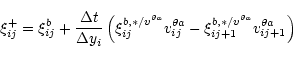 |
(1) |
where
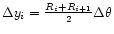 is the "mean
azimuthal width'' of a cell. Equation (1)
expresses the balance of the arbitrary
conservative quantity
in the cell [i,j]by computing the difference of
its inflow at the
[i,j-1]/[i,j] interface
with the velocity
is the "mean
azimuthal width'' of a cell. Equation (1)
expresses the balance of the arbitrary
conservative quantity
in the cell [i,j]by computing the difference of
its inflow at the
[i,j-1]/[i,j] interface
with the velocity
 and its outflow
at the
[i,j+1]/[i,j] interface with the velocity
and its outflow
at the
[i,j+1]/[i,j] interface with the velocity
 .
Actually we consider the flux of the upwinded interfacial quantity
.
Actually we consider the flux of the upwinded interfacial quantity
 ,
where the "
,
where the "
 '' operator depends
on the numerical method (donor cell, van Leer, PPA, see e.g.
Stone & Norman 1992) and on the velocity field
'' operator depends
on the numerical method (donor cell, van Leer, PPA, see e.g.
Stone & Norman 1992) and on the velocity field
 .
.
Up: FARGO: A fast eulerian
Copyright The European Southern Observatory (ESO)