The early stars with H emission we have isolated may have
either intrinsic emission (the objects of our search), or be stars in HII
regions. In the nebulae the central ionizing star visibility in
V band depends on the contribution of the nebula
lines to this band. After spectroscopy of the objects it will be
possible to answer the question, however, examination of
Fig. 2 can considerably clear up the situation. On the plot Hflux -- size for all measured objects of the image No.6 (small circles) the
objects are readily seen to be divided into two (or probably three) branches.
It is natural to connect this division with different morphological
types of the objects: the lower sequence represents "stars'', the upper
(or two upper sequences) -- "nebulae'' or "stars plus nebulae''. On the
image there appeared to be about 60% extended objects, 20% of
stellar objects and also about 20% of the objects
located in the lower-left corner of the diagram of Fig.2 at the point of
a junction of all branches.
emission we have isolated may have
either intrinsic emission (the objects of our search), or be stars in HII
regions. In the nebulae the central ionizing star visibility in
V band depends on the contribution of the nebula
lines to this band. After spectroscopy of the objects it will be
possible to answer the question, however, examination of
Fig. 2 can considerably clear up the situation. On the plot Hflux -- size for all measured objects of the image No.6 (small circles) the
objects are readily seen to be divided into two (or probably three) branches.
It is natural to connect this division with different morphological
types of the objects: the lower sequence represents "stars'', the upper
(or two upper sequences) -- "nebulae'' or "stars plus nebulae''. On the
image there appeared to be about 60% extended objects, 20% of
stellar objects and also about 20% of the objects
located in the lower-left corner of the diagram of Fig.2 at the point of
a junction of all branches.
It is known that a compact HII region can
imitate a hot star in the U-B, B-V colours and may also be a star-like
source (in M33
 pc). Nebulae (or nebulae with
a visible star)
may well be included in the catalogue of hot stars IFM.
For star-like objects the flux must be
pc). Nebulae (or nebulae with
a visible star)
may well be included in the catalogue of hot stars IFM.
For star-like objects the flux must be
 ,
where d is the size of a star on a plate (Zickgraf & Humphreys 1991).
In the case of a supernova remnant or a bubble-type nebula,
,
where d is the size of a star on a plate (Zickgraf & Humphreys 1991).
In the case of a supernova remnant or a bubble-type nebula,
 ,
and in the case of
a filled or a diffuse nebulae,
,
and in the case of
a filled or a diffuse nebulae,
 .
An intermediate power
sequence is also possible depending on the morphology of a nebulae and
a star contribution to the H
band.
.
An intermediate power
sequence is also possible depending on the morphology of a nebulae and
a star contribution to the H
band.
The results of testing this interpretation are contained in Fig. 2.
We plot there from the same image a number of objects, whose morphology is
obvious: apparent but
not bright stars (triangles), large bubble-type nebulae (squares),
"core plus halo''-type nebulae and diffuse nebulae (circles).
The small circles indicate the objects from Fig.1. It is seen from
Fig. 2 that the stars indeed fall in the lower stellar sequence,
bubbles -- in the uppermost sequence (to be more precize, in its
continuation). The third, intermediate sequence is continued by diffuse
and "core plus halo'' nebulae. All three sequences join naturally
in the region of objects' sizes
 .
.
The apparent separation of the objects in Fig. 2 provides grounds to break
up all the studied objects on the basis of their
morphological features in H
into sequences: stars, bubble
nebulae and intermediate diffuse (or complex) nebulae. The objects having low
fluxes and small sizes are common to all three sequences. We label these 4
groups by s, d, b and c, respectively. It should be emphasized that the
division can be done only on the average. Some of the objects fill space
between the sequences, which is caused not only by photometric errors, but by
the real complex morphology of the nebulae.
We made approximations of each of the isolated sequences in Fig.2 with
the inclusion of the objects of known types (bold lines) and only for
the objects under study (thin lines). The objects of type c
were added, when approximating, to all three sequences. For both versions of
the stellar sequence
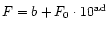 turned out optimum. By
equalling the flux to zero, we find an estimate of the seeing size d0in a given image. In particular, in Fig.2
turned out optimum. By
equalling the flux to zero, we find an estimate of the seeing size d0in a given image. In particular, in Fig.2
 and
and
 for all stars and for the catalogue stars, respectively.
The bubble sequence must satisfy
.
A formal
search for the best curve fitting this data with the power function
 yields
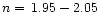 ,
i.e. the square power does fit this type of objects.
Approximations of two samples -- with inclusion of the known bubbles
and without them by
,
i.e. the square power does fit this type of objects.
Approximations of two samples -- with inclusion of the known bubbles
and without them by
 yields a good fit,
a formal seeing estimate is
yields a good fit,
a formal seeing estimate is
 .
.
Approximations of the intermediate type (diffuse) nebulae are also
presented in Fig. 2. One may propose that the appearance of the diffuse
sequence may be due to
inaccuracies in determining the parameters of objects of complex
structure. However, the fact that the bright diffuse nebulae fit well
the intermediate sequence is a forcible argument in favour of reality of the
intermediate objects as a separate diffuse sequence. Approximation of this
sequence by
yields n=3.2 0.3, i.e. the
cubic power describes well the diffuse branch (the formal seeing estimate
there
0.3, i.e. the
cubic power describes well the diffuse branch (the formal seeing estimate
there
 ).
).
It should be noted that the approximation results prove in themselves that we
are working on a nonlinear part of the effective characteristic curve.
We have found that this is valid at least in F < 7000, and practically
all the objects under our study are faint enough to be underexposed.
The images of central region of the galaxy, however, are characterized by a
stronger background and their position on the effective characteristic curve
could be shifted a little to the linear region, where
 .
However the fact that the both fits
(bold and
thin lines in Fig. 2) are very similar gives us a proof that we may
use the approximation
.
However the fact that the both fits
(bold and
thin lines in Fig. 2) are very similar gives us a proof that we may
use the approximation
 for all objects under study.
When examining the rest of the images, we applied quite similar techniques.
The conclusions drawn from a single H
image were confirmed for the
remaining 8. The seeing estimate for all the photographs is
for all objects under study.
When examining the rest of the images, we applied quite similar techniques.
The conclusions drawn from a single H
image were confirmed for the
remaining 8. The seeing estimate for all the photographs is
 ,
which is in agreement with the real seeing value during
the observations (Courtes et al. 1987).
,
which is in agreement with the real seeing value during
the observations (Courtes et al. 1987).
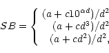 were determined for each sequence
and in each image separately.
were determined for each sequence
and in each image separately.
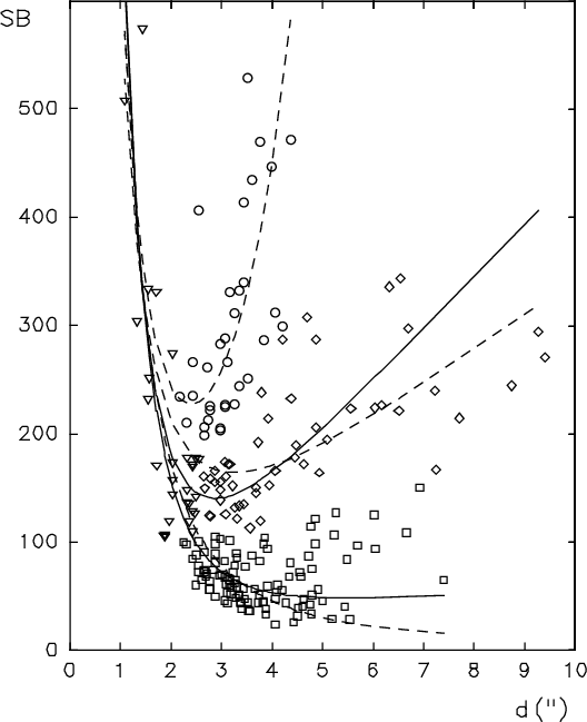
The curves in Fig.3 fit well the sequences (on average),
especially the star sequence -- the upper curve in the figure. Nevertheless
it is quite possible to improve the fits for the extended objects.
For this purpose the photographic effect of a star size growing with star
brightness has to be taken into account. This is most essential for
nebulae of small sizes. From the analysis of Fig.3 it
can be concluded that with nebulae sizes of
 ,
the curves
(two lower dotted lines) overestimate the value
of SB, i.e. the data themselves are located, on average, below the
curves. To allow for this effect, it has to be added to the formula of
the nebulae flux (
,
the curves
(two lower dotted lines) overestimate the value
of SB, i.e. the data themselves are located, on average, below the
curves. To allow for this effect, it has to be added to the formula of
the nebulae flux (
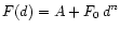 )
a term, which describes the
behaviour of a point-like source,
)
a term, which describes the
behaviour of a point-like source,
 .
Taking
.
Taking
 out of brackets and
expanding the rest into a series with d=d0, one can find that
the allowance for the photographic effect can be made by adding to the
flux expression, a linear term
out of brackets and
expanding the rest into a series with d=d0, one can find that
the allowance for the photographic effect can be made by adding to the
flux expression, a linear term
 .
The solid
lines in Fig.3 show the b and d-type object approximations with
the linear term allowed for. Agreement between the curves and the
data for the nebulae is seen to considerably improved. With the aid of the
diagram SB-d we managed to isolate a part of the objects from the group
c and refer them to one of the three morphological sequences.
.
The solid
lines in Fig.3 show the b and d-type object approximations with
the linear term allowed for. Agreement between the curves and the
data for the nebulae is seen to considerably improved. With the aid of the
diagram SB-d we managed to isolate a part of the objects from the group
c and refer them to one of the three morphological sequences.
Copyright The European Southern Observatory (ESO)
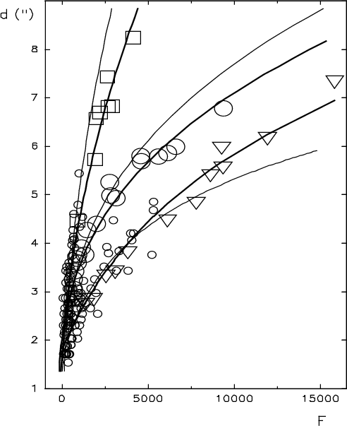
 flux for
the same stars as in Fig. 1 (small circles).
There are also shown
brighter stars (triangles), obvious nebulae -- bubbles (squares) and
diffuses (large circles) from the same image. Bold lines show
approximations of the sequences with bright stars and nebulae included,
thin lines are those for the studied objects only
flux for
the same stars as in Fig. 1 (small circles).
There are also shown
brighter stars (triangles), obvious nebulae -- bubbles (squares) and
diffuses (large circles) from the same image. Bold lines show
approximations of the sequences with bright stars and nebulae included,
thin lines are those for the studied objects only