7 The Mk II auto-folder

Whilst the logical development of the Mk I auto-folder appears to preclude any possibility of refinement, the noisiness of the data raises the possibility that the best fold of any given rotation curve is not necessarily the fold which uses the maximal number of Fourier modes possible for the rotation curve. Thus, for example, the algorithm of Sect. 6.2 might indicate the use of five Fourier modes whilst, in practice, the noisiness of the data might allow a better fold with three Fourier modes.

Thus, given a rotation curve for which a maximum of N Fourier modes are indicated by the data, then the logic of this latter argument forces us to consider a set of potential solutions consisting of the 1-mode fold, the 2-mode fold, ..., the N-mode fold; we must then choose the "best'' solution from this set of N possibilities. Naturally, since the objective quality of the folding process over the whole PS sample is to be judged against the PS solution represented by Fig. 3 left, then the means by which we select between these N folds must be independent of this latter figure. The means by which this is done is described in the following.

   
7.1 Choosing between Fourier modes

The logic of the mode-choosing strategy is rooted in the result of Roscoe 1999A that optical rotation curves are described by the power law $V = A\,R^\alpha$ so that $\ln V$ and $\ln R$ are in a linear relation: Suppose that, for any given rotation curve, we have a choice between Nfolds, consisting of the 1-mode fold, the 2-mode fold, ..., the N-mode fold. For each of these N folds we compute $\ln A$ as described in Sect. 3 (and applying the hole-cutting algorithm described Roscoe 1999A) and, at the same time, record the residual mean square (rms) arising from the regression. We then simply choose the mode which has the least rms associated with it.

In other words, we simply choose the mode that provides the tightest linear fit between $\ln V$ and $\ln R$ after the hole-cutting algorithm has been applied.

7.2 The Mk II auto-folder applied to the PS sample

Applying the Mk II auto-folder described above to the PS sample we find that it gives the $\ln A$ distribution of Fig. 4 right. Comparison with the Mk I solution (Fig. 4 left), shows that the B-peak has strengthened considerably, the C-peak is more-or-less unchanged, the D-peak has weakened slightly whilst the E-peak has strengthed considerably. Thus, the overall impression is that the Mk II auto-folder represents an improvement over the Mk I auto-folder.

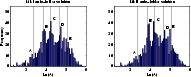Figure 4: Comparison of Mk I and Mk II auto-folder solutions. The vertical lines indicate the positions of the A, B, C, D and E peaks in the PS solution