3 Denoising of CMB maps

3.1 2D wavelet method on a grid

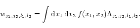
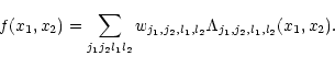
In general for a grid of $2^n\times 2^n$ pixels, a discretization of the parameters of the form: R₁ = 2^{n - j₁}, b₁ =2^{n - j₁}l₁, R₂ = 2^{n - j₂}, b₂ =2^{n - j₂}l₂ for integer-valued j and l allows to introduce the 2D discrete wavelet function

$${\Psi}_{j_1,j_2,l_1,l_2}(x_1, x_2) 2^{(j_1+j_2)/2-n}\psi ( 2^{j_1 - n}x_1 - l_1) \times \psi ( 2^{j_2 - n}x_2 - l_2) \, ,$$ = (12)

where j_i and l_i denote the dilation and the translation indexes, respectively, satisfying $0 \leq j_1 , j_2 \leq n-1, 0\leq l_1 \leq 2^{j_1}-1, 0\leq l_2 \leq 2^{j_2}-1$. The resolution level is defined by $j = \frac{j_1 + j_2}{2}$, corresponding to $R\equiv \sqrt{R_1 R_2} = 2^{n-j}$. We also introduce a scaling function $\phi$ that allows to define a complete basis to reconstruct discrete images,

$${\Phi}_{0,0,0,0}(x_1, x_2) = 2^{- n}\phi ( 2^{- n}x_1 )\phi ( 2^{- n}x_2 ),$$ (13)

$${\Gamma}^{\rm H}_{0,j_2,0,l_2}(x_1, x_2) = 2^{j_2/2 - n}\phi ( 2^{- n}x_1 )\psi ( 2^{j_2 - n}x_2 - l_2),$$ (14)

$${\Gamma}^{\rm V}_{j_1,0,l_1,0}(x_1, x_2) = 2^{j_1/2- n}\psi ( 2^{j_1- n}x_1 - l_1)\phi ( 2^{- n}x_2 ) .$$ (15)

We will consider orthonormal discrete bases as the Haar and Daubechies ones. Denoting by $\Lambda$ any of the previous functions, the orthonormality condition reads:

$$({\Lambda}_{j_1,j_2,l_1,l_2},{\Lambda}_{j_1^{\prime},j_2^{\pr... ...prime}} {\delta}_{l_1l_1^{\prime}}{\delta}_{l_2l_2^{\prime}} ,$$ (16)

where (f,g) denotes the scalar product of two functions in L²(R²).

The wavelet coefficients are now defined by

$$w_{j_1, j_2, l_1, l_2} = \int {\rm d}x_1\,{\rm d}x_2\,f(x_1, x_2) \Lambda_{j_1,j_2,l_1,l_2}.$$ (17)

The image is reconstructed using the following expression:

$$f(x_1, x_2) = \sum_{j_1j_2l_1l_2}w_{j_1, j_2, l_1, l_2} {\Lambda}_{j_1,j_2,l_1,l_2}(x_1, x_2).$$ (18)

A representation of the wavelet coefficients can be done by a square that contains small squares and rectangles associated to different levels of resolution. The first level, representing high-resolution, is j₁ = j₂ = 8 (i.e. j = 8) that contains 65536 wavelet coefficients (each one constructed with $2\times 2 = 4$ pixels for the Haar transform). The second level of resolution contains two boxes: j₁ = 8, j₂ = 7 and j₁ = 7, j₂ = 8 (i.e. j = 7.5) with a total of $2 \times 32768$ wavelet coefficients (each one constructed with $2^2\times 2 = 2\times 2^2 = 8$ pixels for the Haar transform). The levels with j₁ = 0 (or j₂ = 0) contain both contributions from wavelet-wavelet and scaling-wavelet (or wavelet-scaling). Finally, the lower level of resolution is j₁ = j₂ = 0 (i.e. j = 0) and contains four contributions: wavelet-wavelet, wavelet-scaling, scaling-wavelet and scaling-scaling (this last one is proportional to the average value of the image for the Haar transform).

3.2 Reconstruction of CMB maps and radiation power spectra

In the present work we have considered simulated maps of size $12.8^{\circ}\times 12.8^{\circ}$ square degrees, pixel $1.5^{\prime }\times 1.5^{\prime }$ and filtered with a 4.5' FWHM Gaussian beam for a standard CDM model ($\Omega=1$). We have included non-correlated Gaussian noise at different levels (S/N per pixel between 0.7 and 3 at the pixel scale), considering uniform and non-uniform noise. This last case is introduced to account for the non-uniform sampling of satellite observations. As an extreme case we have simulated a noise map with two different regions, one with S/N=3 (approximately one quarter of the map) and a second one with S/N=0.7.

Figure 3: Simulated map of the cosmological signal for the SCDM model (top left), signal plus uniform noise with S/N = 1 (top right), denoised map using wavelets (middle left) and residual map obtained from the CMB signal map minus the denoised one (middle right). For comparison the denoised map using Wiener filter (bottom left) is also shown together with the corresponding residuals (bottom right)

The purpose of the denosing of CMB maps is to reconstruct the original signal map as well as the radiation power spectrum $C_\ell$.

Wavelet decompositions are performed with the package 2D-W developed by our group. The procedure uses two scales, R₁=2^n-j₁, R₂=2^n-j₂, n=9 in our case. High values of j=(j₁+j₂)/2 mean high resolution, i.e., small scales. We distribute the coefficients w_j1,j2,l1,l2 in boxes corresponding to a couple (j₁,j₂), having a total of 81 boxes. The coefficients related to the scaling function are not included in the analysis and they are left untouched. To perform denoising, the basic operation is the comparison between the wavelet coefficients dispersion of the signal in each box with the one of the noise. The Gaussian white noise gives the same contribution in all boxes. Since the signal is negligible at the highest resolutions, the noise dispersion can be directly estimated from the map. Therefore, the signal dispersion can also be estimated for each box.

In Fig. 2, we plot the S/N ratio (defined in terms of the wavelet coefficients dispersions of signal and noise) for each box for a CMB simulation with S/N=1 in real space.

For the case of uniform noise, all boxes where the signal dominates ( $S/N \geq 1.5$) are kept untouched, whereas those with a high level of noise (S/N < 0.3) are removed. On the other hand, the boxes in between are treated with a soft thresholding technique. Given a threshold $\nu$ in terms of the noise coefficients dispersion ( ${\sigma}_n$), the coefficients $\vert w\vert > \nu {\sigma_n}$ are rescaled as $w^{\prime} = w \pm \nu {\sigma}_n$ (where the +, - signs correspond to negative and positive values of w respectively), whereas the remaining coefficients are set to zero. The threshold $\nu$ for each box is chosen using the SURE method (Donoho & Johnstone [1995]). The threshold is obtained by minimization of an unbiased estimate of the expected mean squared error of the estimation of the signal wavelet coefficients (see for instance Ogden [1997]). In Fig. 2, the thresholds obtained with the SURE technique are plotted for a CMB map with S/N = 1. As expected, lower S/N levels are treated with higher thresholds, i.e., more coefficients are removed. Changing the range of S/N where the soft technique is applied (providing is around S/N = 1), does not appreciably change these results. We have used Daubechies 4 but we obtain little or no variations if we adopt higher order Daubechies wavelets. However, the Haar transform gives worse results. Table 1 shows the error in the map reconstructions for different S/N ratios with Gaussian uniform noise. The error improvement achieved with the denoising technique applied goes from factors of 3 to 5 for S/N = 3 - 0.7. The four top panels of Fig. 3 show CMB maps with only signal (SCDM), signal plus noise with a S/N = 1, the reconstructed map using wavelets and the residual one.

Figure 4: Power spectrum of the original CMB (dashed line), CMB plus noise (dotted line) and reconstructed maps using wavelets (solid line) for different levels of noise. Top left panel corresponds to S/N = 0.7, top-right to S/N = 1, bottom-left to S/N = 2 and bottom-right to non-uniform noise (the non-uniform noise map consists in two regions of different S/N ratio; approximately one quarter of the map is at the level of S/N=3 and the rest at S/N = 0.7)

Figure 5: Absolute value of the relative errors of the CMB power spectrum obtained from signal plus noise maps (dotted line), wavelet denoised maps using the SURE thresholding technique (solid line), Wiener denoised maps (dashed line) and wavelet denoised map using a linear method, only on the top-right panel (dot-dashed line). Top-left panel corresponds to S/N = 0.7, top-right to S/N = 1, bottom-left to S/N = 2 and bottom-right to non-uniform noise

   

Table 1: Reconstruction errors (%)

S/N	SURE	linear
0.7	27.4	29.4
1.0	21.7	23.4
2.0	13.3	14.4
3.0	10.0	11.1
N.U.	24.3	-

Regarding non-uniform (N.U.) noise, wavelet techniques allow us to treat each location in the image separately. At each fixed location and fixed (j₁,j₂) we calculate the dispersion of the corresponding noise wavelet coefficient from 500 simulations of our non-uniform noise. Since we consider non-uniform noise that is uncorrelated, the average noise dispersion is the same for all the boxes, as in the uniform noise case. Therefore, we can get again the dispersion of the signal for each (j₁,j₂) pair as well as the S/N ratio for each coefficient. Those coefficients with S/N ratio in the considered range ( $0.3 \le S/N < 1.5$) are treated with a soft thresholding technique, whereas the rest are either kept or removed depending on their S/N ratio. Since in presence of non-uniform noise, we cannot use the SURE technique to estimate the optimal threshold $\nu$ (as far as we know, work is in progress to define a general threshold in the case of non-uniform noise, Von Sachs & McGibbon [1999]), we choose for all the thresholded coefficients $\nu = 1$. This threshold is defined with respect to the noise dispersion in each particular coefficient. We have chosen this value of $\nu$ because it gives a good reconstruction when comparing with the original map, but the results are not very sensitive to the choice of a different threshold in the range $\nu = 0.8 - 2.0$. In Table 1 we present the error of the reconstructed map in the presence of non-uniform noise as considered in this work.

Regarding the power spectrum, $C_\ell$, the denoising method performs very well. Figures 4 and  5 show the reconstructed spectrum and the relative error for $\ell < 2000$ for different S/N ratios (the power spectrum is obtained in the usual way, averaging over the Fourier modes of the considered map at each k). The relative error is $\mathrel{\hbox{\rlap{\hbox{\lower4pt\hbox{$\sim$ }}}\hbox{$<$ }}}$$20\%$ for $\ell < 1700$ in all the considered cases except for the map with S/N = 0.7. In this last case the error increases to $\mathrel{\hbox{\rlap{\hbox{\lower4pt\hbox{$\sim$ }}}\hbox{$<$ }}} 30 \%$ for the same range of $\ell's$.

Finally, we have looked for possible non-Gaussian features introduced by the non-linearity of the soft thresholding technique. We have compared the probability density function of the original and the reconstructed maps using a Kolmogorov-Smirnov test. Both distributions are compatible at similar or higher levels than the original map and the corresponding linear reconstruction obtained with the Wiener Filter technique. Moreover, not significant change is observed in the skewness and kurtosis of the original and reconstructed maps. However, the application of soft thresholding to the wavelet coefficients at a certain level, which are Gaussian distributed for a Gaussian temperature field, clearly changes their distribution by removing all coefficients whose absolute values are below the imposed threshold and shifting the remaining ones by that threshold. Therefore, this technique is introducing a certain level of non-Gaussianity that will depend on the threshold imposed and that should be taken into account when analysing the data. If we are mainly concern about preserving the Gaussian character of the reconstructed image, denoising with wavelet techniques is still possible. Instead of using a soft thresholding technique, we can apply a linear denoising method in wavelet space. In particular, we have removed all wavelet coefficients at boxes with S/N < 1 and left the rest untouched. The reconstruction errors get only slightly worse with this simple linear technique as shown in Table 1. Regarding the reconstructed power spectrum, this is at the same level than the SURE reconstruction (see top-right panel of Fig. 5) for all the considered cases. It is important to remark that the linear denoising method based on 2D wavelets performs much better than the Multiresolution one due to the larger number of boxes corresponding to the product of the 2 scales considered.

3.3 Comparison with other denoising methods

A comparison between Wiener Filter (see for instance Press et al. [1994]) and wavelet techniques has also been performed. In relation to map reconstruction the error affecting the Wiener reconstructed maps is comparable to that achieved with wavelet techniques in all the considered cases. However, in order to apply Wiener filter previous knowledge of the signal power spectrum is required. In a real situation this may well not be possible. The reconstructed and residual maps using Wiener Filter are shown in Fig. 3. In addition, when using Wiener Filter, the power spectrum of the reconstructed image is clearly suppressed at high $\ell's$, giving much worse results than the wavelet technique. For comparison, we have plotted in Fig. 5 the absolute value of the relative error of the $C_{\ell}'s$ for the reconstructions with Wiener Filter. On the other hand, one could recover the $C_\ell$'s of the original signal by subtracting from the power spectrum of the signal plus noise map the estimated power spectrum of the noise, which is constant at each $\ell$. However, this method gives in general worse results than the wavelet techniques and besides cannot be used to reconstruct the image. We have also applied a Maximum Entropy Method to the maps used in this work, with the definition of entropy given by Hobson & Lasenby ([1998]). This method provides reconstruction errors at similar levels as the wavelet techniques. However, we remark that wavelet techniques are computationally faster 0(N) and simpler to apply (not requiring iterative processes) than Maximum Entropy Methods.