3 TSPA with weights

This section contains the detailed formulation of a weighted three stage period analysis for the simple model of Sect. 2.1. The input data $y(t_i)\!\pm\!\sigma_i$ at $t_1 \!\leq \!t_2 \!\leq,..., \leq\!t_n$are $\bar{t}$ (time), $\bar{y}$ (observation) and $\bar{\sigma}$ (error), i.e. the weights are $\bar{w}$, where $w_i\!=\!\sigma_i^{-2}$. The $2K\!+\!2$ free parameters ( $\bar{\beta}$) for our K:th order model

$$g(\bar{\beta}) \! = \! g(t,\bar{\beta}) \! = \! M \! + \! \su... ... \! B_k \cos{ (k2{\pi}ft) } \! + \! C_k \sin{ (k2{\pi}ft) }$$ (1)

are: the mean (M), the amplitudes (B_k, C_k) and the frequency (f), i.e. $\bar{\beta}=[M, B_1,... ,B_K,C_1,..., C_K,f]$. The definition for the phases is $\phi_i\!=\!{\mathrm{FRAC}}[ft_i]$, where FRAC removes the integer part of ft_i. The TSPA consists of three consecutive stages: the pilot- (PSch), the grid- (GSch) and the refined-search (RSch).

   
3.1 Pilot Search (PSch)

The order K (Eq. 1) determines the PSch "model'' $\tau$ (Eq. (2) below). The PSch searches for the best period "candidates'' over a long interval between P_min ( f_max^-1) and P_max ( f_min^-1). Typical correlation lengths in time ( D_min, D_max) and phase ($\tau$) are , $D_{\mathrm{min}} \! \approx \! 0.9 P_{\mathrm{min}}$, and

  $$\tau = (4K)^{-1}.$$

Note that only $\tau$ is connected to our model (Eq. 1). The consequences of and the reasons for selecting adjustable correlation lengths D_min, D_max and $\tau$ are discussed in the end of this section, as well the particular connection between $\tau$ and the modelling order K (see also the beginning of Sect. 3.2).

The PSch uses four sets of $N\!=\!n(n-1)/2$ pairs: t_i,j, y_i,j, w_i,j and $\phi_{f,i,j}$( $i\!=\!1,... ,n-1$ and $j\!=\!i\!+\!1,... ,n$). The first three, $t_{i,j}\!=\ \mid \!t_i\! - \!t_j \! \mid$, $y_{i,j}\!= \! [ y(t_i)\! - \! y(t_j)]^2$ and $w_{i,j}\!= \! (w_iw_j) (w_i\!+\!w_j)^{-1}$, are independent of f, but the ${\phi}_{f,i,j}\!=\!{\mathrm{FRAC}} [ f t_{i,j}]$ are not. The PSch periodogram determined at all integer multiples of ${\Delta}f_{\mathrm{pilot}}\!=\![10D_{\mathrm{max}}]^{-1}$ between f_min and f_max is

$${\Theta}_{\mathrm{pilot}}(f) = { {\sum_{i=1, j=i+1}^{n-1,n} ... ...{i=1, j=i+1}^{n-1,n} Z(\phi_{f,i,j}) ~W(t_{i,j}) ~w_{i,j}} },$$ (3)

where

$$Z({\phi}_{f,i,j}) =$$ (5)

The following algorithm is efficient for larger samples of data, because it eliminates the problem that the number of t_i,j, y_i,j, w_i,j and $\phi_{f,i,j}$increases with $\propto\!n^2$.

1.

Because W(t_i,j) does not depend on f(Eq. 4), apply this function only once.

2.

Divide $D_{\mathrm{min}}\!\leq\!t_{i,j}\!\leq\!D_{\mathrm{max}}$into $J\!=\!{\mathrm{INT}}[(D_{\mathrm{max}}-D_{\mathrm{min}}) {\Delta}^{-1}]+1$ bins ($J\!\ll\!N$ for larger samples), where the bin width is $\Delta\!=\!10^{-1}P_{\mathrm{min}}$ and INT removes the decimal part of $(D_{\mathrm{max}}-D_{\mathrm{min}}) {\Delta}^{-1}$.

3.

Denote the n_q values of t_i,j, y_i,j and w_i,j in the q:th bin by t'_k, y'_k and w'_k. Derive $t'_q\!=\! n_q^{-1} \Sigma_{k=1}^{n_q} t'_k$, $y'_q\!=\! [\Sigma_{k=1}^{n_q} w'_k]^{-1} \Sigma_{k=1}^{n_q} w'_k ~y'_k$and $w'_q\!= \! \Sigma_{k=1}^{n_q} w'_k$ for every bin.

4.

Calculate the modified PSch periodogram

where Z (Eq. 5) is applied to ${\phi}'_{f,q}\! =\! {\mathrm{FRAC}}[ f t'_q]$.

This algorithm divides the data into J bins with respect to the time differences t_i,j between D_min and D_max. The original t_i,j, y_i,j and w_i,j data are replaced by the J averages t'_q, y'_q and w'_q within these bins. The algorithm is efficient, because the Z function in Eq. (6) has to applied only to J ($\ll N$) values at each tested f.

The y_i,j differences closer than $\tau$ in $\phi_{f,i,j}$are smaller for a good f candidate, i.e. the data form a continuous curve. Such f minimize the PSch periodogram (Eqs. 3 or 6), the case being opposite for poor f candidates. Because W(t_i,j) (Eq. 4) excludes y_i,j too far in t_i,j, phase shifts during time intervals longer than D_max do not influence the periodogram. The combination of $D_{\mathrm{max}}\!=\!\Delta T\!$ and $D_{\mathrm{min}}\!=\!0$ would include all data (Eq. 4), but D_min is applied, because y_i,j do not contain significant information when t_i,j goes below P_min. Adjusting D_min and D_max determines the number of y_i,j selected with W(t_i,j). The function $Z(\phi_{f,i,j})$ selects only $y_{\rm {i,j}}$ closer than $\tau$ in $\phi_{f,i,j}$ (Eq. 5). For example, $\tau\!=\!0.25$ determines a sinusoidal model (Eqs. 1 and 2). The y_i,j on a sinusoid correlate within $\phi_{f,i,j}\!=\!\pm 0.25$, or those on a double wave ($K\!=\!2$) within $\phi_{f,i,j}\!= \!\pm 0.125$. Reduction of $\tau$ enables detection of more complex $\bar{y}$ variation, but reduces the number of y_i,j selected with $Z(\phi_{f,i,j})$, i.e. requires more data.

Figure 1: The second order TSPA for SET=42 ($n\!=\!149$): a) $\Theta'_{\mathrm{pilot}}(f)$ (Eq. 6) is the PSch periodogram between $P_{\mathrm{min}}\!=\!0.5$ and $P_{\mathrm{max}}\!=\!10$ with correlation lengths $D_{\mathrm{min}}\!=\!0.45$, $D_{\mathrm{max}}\!=\!30$ and $\tau\!=\!0.125$. The number of independent frequencies is $m\!=\!55$ (Eq. 9). The diamonds on $\Theta_{\mathrm{pilot}}(f)$mark the five best periods P1, ..., P5. b-f) The $y_i(\phi _i)$ with these P1, ..., P5. g-k) The diamonds on $\Theta_{\mathrm{grid}}(f)$ (Eq. 7: $K\!=\!2$) indicate the more accurate P1, ..., P5 obtained with the GSch. l-p) RSch determines the final P1, ..., P5, and their $P(\chi ^2_0)$ (Eq. 10). The continuous lines connect each $(\phi _i, y_i)$ to the closest point of the model $(\phi ,g(\phi ))$. q-u) The $\delta \phi '_i$ versus $\delta \phi _i$(see end of Sect. 5) of each P1, ..., P5 for $P_0\!=\!0.9997$ given by $\gamma_{\mathrm{n}}$ (Eq. 15). The critical levels for the linear correlations between $\delta \phi '_i$ and $\delta \phi _i$ are $P(\mid\!r_0\!\mid)$

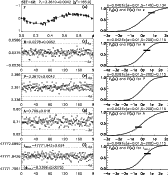Figure 2: The $S\!=\!200$ RSch bootstrap of SET=42: a) The model ($\bar{g}$) with $P_1\!=\!3.3610 \!\pm 0.0042$ already shown in Fig. 1l. b) The FS(u) and F(u) (Eqs. 12 and 13) for the $S\!=\!149 (=\!n)$ residuals $\bar{\epsilon}$ confirm a Gaussian distribution (i.e. HG is not rejected with $\alpha \!=\!0.01$in Eq. 14). A dark rectangle indicates the location and height of the Kolmogorov-Smirnov test statistic ( $a = {\mathrm{max}} [~\mid F_{\mathrm{S}}(u)- F(u) \mid~]$). c and d) The $S\!=\!200$ bootstrap M estimates (open squares) also follow a Gaussian distribution. e-j) The same as in c and d) for the P, A and tmin,1 estimates

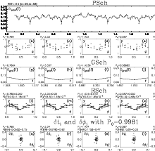Figure 3: Same as in Fig. 1 for SET=114

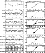Figure 4: Same as in Fig. 2 for SET=114. Note: e and f) $H_{\rm G}$ is rejected for P (Eq. 14). k) Only $S\!=\!163$ estimates are obtained for tmin,2. The bootstrap samples with no tmin,2 are marked with vertical lines

   
3.2 Grid Search (GSch)

The PSch over a long f interval usually detects numerous frequency "candidates'' f'. More accurate values for at least five best f' are determined with the GSch. The TSPA applications for real data may sometimes require testing of a much larger number of f' detected with the PSch. Here the limit of testing only the five best f' was chosen, because it is convenient for the graphical representation of the results, like in Figs. 1, 3, 5 and 7. The PSch "model'' $\tau$ can not fully constrain the modelling order K (Eqs. 1 and 2), because y_i,j closer than $\tau$ in $\phi_{f,i,j}$ may correlate in several different models. For example, the PSch could detect a box function or a sinusoid with $\tau\!=\!0.25$. The model is fixed in the GSch, e.g. if $\tau\!=\!0.25$, GSch proceeds with a $K\!=\!1$ model (Eq. 1). If PSch detects f', then GSch tests all integer multiples of ${\Delta}f_{\mathrm{grid}}\!=\![G]^{-1} f_0$between $f' \! - \! 5 {\Delta}f_{\mathrm{pilot}}$ and $f' \! + \! 5 {\Delta}f_{\mathrm{pilot}}$, where $G\!\geq\!10$ is called the "overfilling factor'' and $f_0\!=\! (\Delta T)^{-1}$. The discrete tested f set within this narrow interval is denser than in the PSch (i.e. ${\Delta}f_{\mathrm{grid}}\!\leq\!{\Delta}f_{\mathrm{pilot}}$). Standard linear least squares fits to $\bar{y}$ with $\bar{w}$for every tested f in Eq. (1) (i.e. f is not a free parameter) determine the GSch periodogram

$${\Theta}_{\mathrm{grid}}(f) = 2 \left[ \sum_{i=1}^n w_i \ri... ..._{i=1}^n ~w_i \left[ y(t_i)-g(t_i,\bar{\beta}_f) \right]^2,$$ (7)

where $\bar{\beta}_f\!=\! [M,B_1,...,B_K,C_1,...,C_K]$ minimizes the residuals $\epsilon_i \!=\!y(t_i)\!-\!g(t_i,\bar{\beta}_f)$(note that $\Theta_{\mathrm{grid}} \! \neq \! \chi^2$), and the factor 2 adjusts $\Theta_{\mathrm{grid}}$ to the quantitative level of $\Theta_{\mathrm{pilot}}$. Thus the PSch periodogram with $\tau\!=\!(4K)^{-1}$ represents an approximation of the GSch periodogram with K.

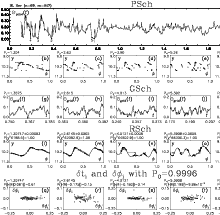Figure 5: The fifth order TSPA ($K\!=\!5$) for the V magnitudes of the cepheid variable BL Her, otherwise as in Fig. 1

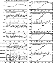Figure 6: The $S\!=\!200$ fifth order RSch bootstrap with $P_1\!=\!1.307465$ for the V magnitudes of BL Her, otherwise as in Fig. 2. Note: k) Only $S\!=\!190$ estimates are obtained for tmin,2

Figure 7: The first order TSPA ($K\!=\!1$) between $P_{\mathrm{min}}\!=\!0.4$ and $P_{\mathrm{max}}\!=\!50$ for the V magnitudes of SAO50205 during subsets SET=111, 112, 113 and 114, otherwise as in Fig. 1

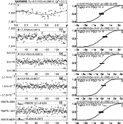Figure 8: The $S\!=\!200$ first order RSch bootstrap with $P_2\!=\!0.51452$for the V magnitudes of SAO50205, otherwise as in Fig. 2

   
3.3 Refined Search (RSch)

The model (Eq. 1) is nonlinear when f is a free parameter. The RSch performs a standard Marquardt iteration (e.g. Press et al. 1988) to compute $\bar{\beta}$. But the result of this iterative refinement depends on the trial solution ( $\bar{\beta}_0$). Large discrete f sets are tested with PSch and GSch only to provide a reliable $\bar{\beta}_0$ for RSch. Combining the f' detected in the GSch to $\bar{\beta}_{f'}$ (Eq. 7) gives $\bar{\beta}_0 =[\bar{\beta}_{f'},f']$. While the PSch and GSch test discrete f sets, the RSch is continuous in f, because it utilizes the analytical properties of

$$\chi^2 (\bar{\beta}_{\mathrm{min}}) = \sum_{i=1}^n w_i \left[y(t_i)-g(t_i,\bar{\beta}_{\mathrm{min}})\right]^2,$$ (8)

where $\bar{\beta}_{\mathrm{min}}$ minimizes the $\chi^2$. This $\chi^2$ enables significance estimates. The number of independent frequencies (m) determines how many independent $\chi^2$-tests are done with the model of Eq. (1). Since the TSPA is performed between f_min (P_max^-1) and f_max (P_min^-1), a logical definition is

$$m \!=\! {\mathrm{INT}} [(f_{\mathrm{max}}-f_{\mathrm{min}})f_0^{-1}],$$ (9)

where $f_0\!=\!\Delta T^{-1}$. This definition is equivalent to that in Jetsu & Pelt (1996, Eq. 13), who presented an empirical approach to verify Eq. (9) (see also Buccheri & De Jager 1989). To understand the connection between f₀ and m, consider an arbitrary test statistic z(f) that depends on $\phi_i\!=\!{\mathrm{FRAC}}[ft_i]$. Because $\Delta T (f \pm f_0) \!-\! \Delta T f \!=\!\pm1$ for any f, the correlation between z(f) values vanishes within f₀ when the $\phi_i$ order is totally rearranged. An overfilling factor, e.g. $G \! \ge \! 10$ in GSch, enables more accurate period determination, but does not deteriorate the statistics, i.e. testing many frequencies within $\pm f_0/2$ amounts to testing only one independent frequency. Hence the TSPA performs m independent $\chi^2$-tests over the frequency interval [f_min,f_max]. Our "null hypothesis'' is:

H₀: The data are pure noise.

Under H₀, the probability (i.e. the critical level) for reaching a particular, or an even smaller, $\chi^2_0$ value, is

$$P(\chi_0^2)\!=\!P(\chi^2 \!\leq\! \chi_0^2, \nu, m) \!=\!1\!-[1-P(\chi^2 \!\leq\! \chi^2_0)]^{\mathrm{m}},$$ (10)

where $\nu\!=\!n\!-\!(2K+2)$ is the degree of freedom for $\chi^2$. The validity of $\chi^2$ statistics is verified in the next section by testing the hypothesis that the model residuals and parameters have a Gaussian distribution.