4 Discussion

4.1 Phase measurements

Phase measurements have to be performed in two wavebands for fringe tracking with air-filled delay lines, and the useful quantity or "observable'' is their difference. In each band, phase is continuously changing with the air delay, typically 2 rad per meter, so that the measured phase is not constrained. Two schemes can be considered, for beam combination in a pupil plane:

• optical path modulation, at a fast enough rate to freeze the atmospheric turbulence,
• simultaneous in-phase and quadrature-phase measurements.

1) Optical path modulation has been implemented on the first interferometer prototype for optical astrometry (Shao & Staelin 1980), and later on the MkIII interferometer (Shao et al. 1988), with one wavelength stroke and 4-quadrants measurements. The problem of fringe ambiguity was partly solved with the two-color method which, in the visible, greatly reduced the atmospheric piston effect (Colavita et al. 1987). A more sophisticated technique, with channeled spectrum and delay modulation is implemented on NPOI (Armstrong et al. 1998). This technique gives the fringe amplitude and phase as function of wavenumber. Due to the larger wavelength range of the instrument, about an octave, the stroke is twice the mean wavelength, with 8 samples per scan length. Both with MkIII and NPOI, a single output of the beam combiner is used for fringe measurement. Another approach is to have a 2-quadrants optical path modulation ($0, \lambda/4$)with simultaneous measurements of the two complementary outputs of the beam combination (Tango & Twiss 1980).

  

Figure 5: Basic principle of the two-beam combination in pupil plane, with 4 output phases and wide bands

2) Simultaneous in-phase and quadrature-phase measurements can be obtained with two combinations as shown in Fig. 5, and a $\pi/2$ phase shift in one of the interferometer arm for the quadrature-phase combination. Phase measurements being performed in two different wavebands, the phase shift has to be achromatic which is possible with a polarization splitter and two total reflections in glass material, e.g. an achromatic Fresnel rhomb retarder.

4.2 Signal/Noise ratio

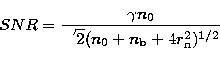
We compare the sensitivity for phase measurements in a single band, either with path length modulation and 4-quadrants measurements (scheme 1), or with quadrature-phase combination (scheme 2). Let I₀ the incoming source flux, in each interferometer arm, and T₀ the 4-steps scan duration in scheme 1 or the integration time in scheme 2. Neglecting instrumental losses, the number of useful photons per measurement and per arm is n₀=I₀T₀. With equal intensity splitting before beam combinations, the 4 outputs of Fig. 5 are, in each band:

$$J_{k} = \frac{n_{0}}{2} [1+\gamma\cos(\phi + \theta_{k})]$$ (31)

with $\theta = [-\pi/2, \pi/2, 0, \pi]$.

The useful quantities for phase measurements are: Let $n_{\rm b}$ the background photons number (from a single arm, during T₀), and the readout noise variance. With Poisson statistic for the photons, the total noise variance per X or Y measurements, each with two reads, is $b^{2} = n_{0}+ n_{\rm b}+ 2 r^{2}_{\rm n}$, and the SNR of phase measurements is:

$$SNR = \frac{\gamma n_{0}}{( n_{0}+ n_{\rm b}+ 2r^{2}_{\rm n})^{1/2}}\cdot$$ (32)

With a 4-steps optical path modulation and a single output in the beam combination (e.g. MkIII), the achievable SNR would be:

$$SNR = \frac{\gamma n_{0}}{\sqrt{2}( n_{0}+ n_{\rm b}+ 4r^{2}_{\rm n})^{1/2}}$$ (33)

the $\sqrt{2}$ loss factor in the denominator being recovered if the two complementary outputs are simultaneously used. For weak sources, with readout as dominant noise factor, the 4-steps modulation scheme is less sensitive than our proposed scheme, whereas a 2-steps path modulation scheme (0, $\lambda/4$) and detection of the two complementary outputs will give the same figure of merit.

In this sensitivity estimate, we have considered only photon noise and readout noise. In a real situation, visibility fluctuations due to phase corrugations of the wavefront (e.g. Lawson et al. 1999) should be considered as additional atmospheric noise in SNR estimates with optical path modulation. On the other hand, only scintillation noise has to be added in the average SNR estimate of the quadrature-phase scheme, n₀ being replaced by $n_{0}(1+\sigma_{I}^{2})$ in the denominator of (32) where $\sigma_{I}$ is the scintillation index, as seen by the detector.

4.3 Longitudinal dispersion and leading wavenumber

The value of the leading wavenumber is not measured directly, it is deduced from the effective guiding pair ($\tilde \sigma_1, \tilde \sigma_2$). The relative uncertainty on group delay, and hence on astrometric precision is, with the $(K_{\rm s},H)$ pair and conditions prevailing at Paranal: $\epsilon_{L} \simeq 2\ 10^{-6}\epsilon_{\sigma}$ where $\epsilon_{\sigma}$ is the relative uncertainty on the leading wavenumber. That is to say the simple model used here for the air refractive index will be adequate for reaching single-field astrometric precision of a few milliarcseconds, or a few parts in 10⁸. For dual-field operations, the uncertainty requirement on differential delay is much more stringent, about one part in 10¹⁰, that is $\epsilon_{\sigma} \leq 10^{-4}$. It means that the light beams from the two observed stars have to cross as much as possible the same dispersive media, band filters, and more generally optical parts. This is why we are investigating a time multiplex scheme for dual-field astrometry, phase measurements in one or the other field being performed without optical path modulation.

With added glass compensation plates, the situation may not be so simple for astrometric calibration of the instrument. Relation (25) for the glass refractive index might not be realized exactly, a consequence being uncontrolled variations of the leading wavenumber $\sigma_{0}$ with delay length.

4.4 Group delay versus residual phase measurements

For group delay tracking, the "observable'' quantity is a difference in residual phase between two wavebands $\sigma_{1}$ and $\sigma_{2}$, and the residual group delay is vanishing for the leading wavenumber $\sigma_{0}$. In the approximation made for the air refractive index, keeping only the $\sigma^{2}$ term in its development, the $\sigma_{0}$ value is not dependent on the ambient parameters, and the approximation is valid to a few parts in 10³, neglecting the water vapor contribution.

On the other hand, the residual phase in the two wavebands $\sigma_{1}$ and $\sigma_{2}$ is, with (17) and (20):

$$\phi_{1,2} = 2\pi\sigma_{1} \sigma_{2} (\sigma_{1}+\sigma_{2}) \beta L_\mathrm{del}.$$ (34)

The sensitivity to path length variations of $\phi_{1}+\phi_{2}$ is larger than the sensitivity of group delay measurement, the gain factor being $(\sigma_{1} + \sigma_{2})/(\sigma_{1} - \sigma_{2})$, that is about 7.5 for the ($K_\mathrm{s}, H)$pair. Once coherencing is achieved, optical path delay tracking with phase locking in one or the other waveband could be used, in a more sensitive way than group delay tracking alone. But a model for the residual phase variations with air delay length is needed, so that the interest of phase locking has to be demonstrated with a real experiment.

Group delay tracking will operate only with a significant SNR in each wavebands, say larger than 5. The uncertainty in the phase difference will then be smaller than $0.2\,\sqrt{2}$ rad, or about 16 degrees per individual measurement. With about 50 measurements per second, a 1 degree rms value, or 20 nm with the ($K_\mathrm{s}, H)$ pair, is reached after 5 seconds of observing time. Such a sensitivity to path length variations is considered to be good enough for conveniently averaging the atmospheric piston in single-field astrometry, the duration of each observing sequence being larger than a few 10 seconds. For dual-field astrometry with two bright sources, the sensitivity in differential atmospheric piston will be $\sqrt{2}$ times the previous figure, that is better than 10 nm in a 45 s observing sequence, or better than 0.1 mas/sequence with a 30-40 m baseline, which is also considered as a consistent sensitivity figure.