

Up: Astrometric optical interferometry with
Subsections
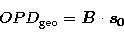
The atmosphere is first supposed to be a stratified medium
without turbulence. The baseline  is horizontal,
and much shorter than the scale height of the atmosphere. Let
is horizontal,
and much shorter than the scale height of the atmosphere. Let  the
refractive index of the atmosphere at the interferometer level,
and
the
refractive index of the atmosphere at the interferometer level,
and  the wavenumber or inverse of the wavelength,
  the source
direction as seen by the instrument. The Optical Path
Delay of the rays at the two entrance pupils, or geometrical OPD, is the scalar
product
the source
direction as seen by the instrument. The Optical Path
Delay of the rays at the two entrance pupils, or geometrical OPD, is the scalar
product  . With the Snell's law on ray
propagation, this quantity keeps to be the same all along the ray path through the
atmosphere, and it equals its value outside the atmosphere:
. With the Snell's law on ray
propagation, this quantity keeps to be the same all along the ray path through the
atmosphere, and it equals its value outside the atmosphere:
|  |
(1) |
where  is the source direction outside the atmosphere, or without
refraction. The quantity
is the source direction outside the atmosphere, or without
refraction. The quantity  is also the geometric group
delay for the propagation of wavepackets.
is also the geometric group
delay for the propagation of wavepackets.
For wave propagation through an isotropic dispersive medium, two features have to be
considered:
- propagation of lateral coherence, or of wave surfaces normal to the ray paths.
The phase variation between two points P1 and P2 along a ray path is
proportional to the optical length
 between this two points with:
| 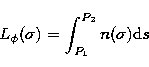 |
(2) |
- propagation of longitudinal coherence, or of wavepackets. Between two points
P1 and P2 along a ray path, the group delay is:
| 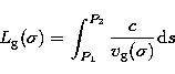 |
(3) |
where  is the group velocity:
| ![\begin{displaymath}
v_\mathrm{g} = \frac{c}{n(\sigma)}\, \left[1 - \frac{\sigma}{n(\sigma)}\,\frac{\partial
n} {\partial \sigma}\right].\end{displaymath}](/articles/aas/full/1999/14/ds1718/img16.gif) |
(4) |
In a weakly dispersive medium such as the air, we shall have:
| ![\begin{displaymath}
\frac{c}{v_\mathrm{g}(\sigma)} \simeq n(\sigma)\,\left[1 + \...
...\sigma}{n(\sigma)}\,
\frac{\partial n}{\partial \sigma}\right] \end{displaymath}](/articles/aas/full/1999/14/ds1718/img17.gif) |
(5) |
and in the visible and near-IR range, the difference between optical length and group
delay is as small as a
few parts in 106. Nevertheless the use of OPD for the whole optical path within
the interferometer with non-evacuated pipes is ambiguous. Does it stand for optical
length or for group delay? so that we shall use it only for the geometrical delay
outside the interferometer, eventually affected by the fluctuations of the atmospheric
piston:
| 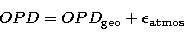 |
(6) |
the long term average of the last quantity being zero.
With an evacuated delay line with length ,the basic equation for the residual optical length of the interferometer is:
|  |
(7) |
As long as the interferometer "offset''  is achromatic or non
dispersive, there exists a fringe with zero phase at any wavenumber. The
"white-fringe'' is obtained for
is achromatic or non
dispersive, there exists a fringe with zero phase at any wavenumber. The
"white-fringe'' is obtained for  . This is also the condition for
zero group delay, so that the maximum coherence is obtained at the white-fringe, and
all these are well-known results for an optical interferometer with evacuated delay
line.
. This is also the condition for
zero group delay, so that the maximum coherence is obtained at the white-fringe, and
all these are well-known results for an optical interferometer with evacuated delay
line.
The interferometer offset will not be further considered in this paper, and dropped to
zero in the following. A delay line with length  located in an
air-filled tunnel will compensate exactly the OPD at a single wavelength only.
Furthermore two types of compensation are obtained, either optical length compensation
or group delay compensation, the residual lengths being respectively given by
located in an
air-filled tunnel will compensate exactly the OPD at a single wavelength only.
Furthermore two types of compensation are obtained, either optical length compensation
or group delay compensation, the residual lengths being respectively given by  and
and  with:
with:
|  |
(8) |
| (9) |
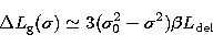
and with (5):
| ![\begin{displaymath}
\Delta L_\mathrm{g}(\sigma) = OPD - \left[n(\sigma) + \sigma \frac{\partial n}{\partial
\sigma}\right] L_\mathrm{del}.\end{displaymath}](/articles/aas/full/1999/14/ds1718/img26.gif) |
(10) |
The residual phase being  , the relation between
residual phase derivative and residual group delay is easily checked:
, the relation between
residual phase derivative and residual group delay is easily checked:
|  |
(11) |
Coherencing, or group delay tracking with  , has to be
performed at a peculiar wavenumber determined
by the instrumental set-up. Let
, has to be
performed at a peculiar wavenumber determined
by the instrumental set-up. Let  its value, and
  the
wavenumber with zero residual phase, it is solution of:
the
wavenumber with zero residual phase, it is solution of:
|  |
(12) |
The air refractive index being an increasing function wrt wavenumber,
 .
.
There is no simple analytical form for the air refractive index in a wide optical
range. Fits to index measurements lead to the following general expression in terms of
the wavenumber (see e.g. Owens 1967):
|  |
(13) |
where the coefficients are dependent on the partial pressures of the minor components
(water vapor, carbon dioxyde, ...), and on temperature and total pressure.
In the near-IR range, with  , only a few terms in a
 power expansion of the preceeding expression are to be considered. With
the additional assumption of the dry component and wet air component obeying the ideal
gas law, both separately and for the combined mixture, a dry air refractive index
expansion is given by Gubler & Tytler (1998):
power expansion of the preceeding expression are to be considered. With
the additional assumption of the dry component and wet air component obeying the ideal
gas law, both separately and for the combined mixture, a dry air refractive index
expansion is given by Gubler & Tytler (1998):
|  |
(14) |
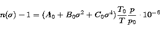
with A0 = 287.604, B0 = 1.6288, C0 = 0.0136, and standard conditions
T0=273.15 K and p0=1013.25 hPa.
In this paper, the numerical applications will be performed for the atmospheric
conditions prevailing in the VLTI interferometer tunnel, i.e. T=289 K and
p=743 hPa (Lévêque 1997), so that (14) reduces to:
|  |
(15) |
with 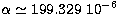 ,
, 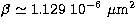 and
and 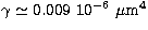 .
.
To better than a few parts in 103 and for better clarity, we shall neglect the
 term in the analytic developments of the air dispersive effect. The
contribution of water vapor to dispersion effects may be difficult to modelize in the
near-IR transmission bands, that is in the vicinity of water vapor absorption bands.
With the conditions prevailing in the VLTI tunnel, its contribution, although small,
is not known exactly and should be measured and monitored during astrometric
observations.
term in the analytic developments of the air dispersive effect. The
contribution of water vapor to dispersion effects may be difficult to modelize in the
near-IR transmission bands, that is in the vicinity of water vapor absorption bands.
With the conditions prevailing in the VLTI tunnel, its contribution, although small,
is not known exactly and should be measured and monitored during astrometric
observations.
![\begin{figure}
\includegraphics [width=8cm,clip]{ds1718f1.eps}\end{figure}](/articles/aas/full/1999/14/ds1718/Timg43.gif) |
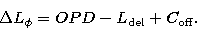
Figure 1:
Residual phase and residual group delay per meter of
air-filled delay line, and for the 3 pairs of guiding wavenumbers (see
Table 1). Zero group delay is shown as a (*) on each curve. The near-IR
wavebands with 15% relative width are also shown (full segments) |
The departure to a white-fringe, with zero residual phase and group delay, is due to
the  term in the simplified expression for the refractive index, and
the solution to (12) is:
term in the simplified expression for the refractive index, and
the solution to (12) is:
|  |
(16) |
The residual phase is an odd cubic function of the wavenumber given by:
|  |
(17) |
with its maximum at  . Equal phase can be measured at two different
wavenumbers
. Equal phase can be measured at two different
wavenumbers  and
and  with
with  ,and this property will be used in the proposed fringe tracking system. Residual phase
is plotted in Fig. 1 for 1 meter of delay line, and for three
different values of , ranging from the K band to the H band.
,and this property will be used in the proposed fringe tracking system. Residual phase
is plotted in Fig. 1 for 1 meter of delay line, and for three
different values of , ranging from the K band to the H band.
The residual group delay is:
|  |
(18) |
that is  for zero residual phase, or a few
 m per meter of delay line. The residual group delay is plotted in
Fig. 1 for the three different values. It is seen also
as the slope of the phase curves.
m per meter of delay line. The residual group delay is plotted in
Fig. 1 for the three different values. It is seen also
as the slope of the phase curves.
Up: Astrometric optical interferometry with
Copyright The European Southern Observatory (ESO)
![\begin{figure}
\includegraphics [width=8cm,clip]{ds1718f1.eps}\end{figure}](/articles/aas/full/1999/14/ds1718/img43.gif)