Up: Atomic data from the
Subsections
The resulting effective collision strengths for the electron-temperature range
 are listed in Table 6.
We have used an R-matrix basis of 25 continuum orbitals,
adequate for electron collision energies up to 200Ryd.
In the following sections each of the effects mentioned in Sect. 2 is
discussed in detail.
The low-energy regime of the collision strengths
for a highly ionized system such as Fe XVI is dominated
by series of very narrow resonances. It would be computationally expensive to
calculate such cross sections with an energy mesh fine enough to
resolve all these features.
However a practical choice must
ensure stable integration when the rates are calculated.
This is illustrated in Fig.1, where the effective collision
strength for the transition 3d
are listed in Table 6.
We have used an R-matrix basis of 25 continuum orbitals,
adequate for electron collision energies up to 200Ryd.
In the following sections each of the effects mentioned in Sect. 2 is
discussed in detail.
The low-energy regime of the collision strengths
for a highly ionized system such as Fe XVI is dominated
by series of very narrow resonances. It would be computationally expensive to
calculate such cross sections with an energy mesh fine enough to
resolve all these features.
However a practical choice must
ensure stable integration when the rates are calculated.
This is illustrated in Fig.1, where the effective collision
strength for the transition 3d D
D S1/2 has
been plotted when computed with different mesh sizes. By comparing
results obtained with steps of
S1/2 has
been plotted when computed with different mesh sizes. By comparing
results obtained with steps of  Ryd
and
Ryd
and  Ryd (z=15 is
the residual charge of the ion), it is concluded that the latter mesh size is
sufficiently fine while a mesh with a step of
Ryd (z=15 is
the residual charge of the ion), it is concluded that the latter mesh size is
sufficiently fine while a mesh with a step of  Ryd can lead to significant differences at the lower temperatures. Therefore
cross sections are computed in the energy region below the highest threshold
(
Ryd can lead to significant differences at the lower temperatures. Therefore
cross sections are computed in the energy region below the highest threshold
( ) with a step of
  10-5 Ryd. In the region
where all channels are open a wider step of
10-5 Ryd. In the region
where all channels are open a wider step of  Ryd is more than adequate.
![\begin{figure}
\includegraphics []{8187f1.eps}\end{figure}](/articles/aas/full/1999/08/ds8187/Timg74.gif) |
Figure 1:
Effective collision strength for the
3dD5/2-4s transition in Fe XVI computed
with different energy meshes. Crosses: Ryd.
Asterisk: Ryd. Circles:
Ryd. The residual charge of the system is transition in Fe XVI computed
with different energy meshes. Crosses: Ryd.
Asterisk: Ryd. Circles:
Ryd. The residual charge of the system is
 . It may be seen that the latter two meshes lead to stable
integration throughout the whole temperature region . It may be seen that the latter two meshes lead to stable
integration throughout the whole temperature region |
As mentioned in Sect. 2, relativistic contributions are taken into account
by either of two methods: by diagonalizing the Hamiltonian in intermediate
coupling
using a Breit-Pauli approximation,
or, with less effort, by calculating reactance matrices in LS coupling before
transforming to pair coupling using algebraic coefficients and TCCs.
It is found that, for most transitions, effective collision
strengths computed with the two methods are in good agreement. However
for some transitions, particularly those arising within a term,
the differences at low temperatures can be sizable as shown in Fig. 2. This
is mainly caused by the neglect of the term energy
splittings in the TCC method; i.e. energy-degenerate channels give rise to
significantly
different resonance patterns. Therefore it is advisable to adopt the full
Breit-Pauli approach whenever possible.
![\begin{figure}
\includegraphics []{8187f2.eps}\end{figure}](/articles/aas/full/1999/08/ds8187/Timg76.gif) |
Figure 2:
Effective collision strength for the
3pP pP pP transition in Fe XVI
showing a large difference at low temperatures when the relativistic
contributions are taken into account with the TCC method (crosses) and a
Breit-Pauli calculation (circles) transition in Fe XVI
showing a large difference at low temperatures when the relativistic
contributions are taken into account with the TCC method (crosses) and a
Breit-Pauli calculation (circles) |
By comparing effective collision strengths computed with Options 0 and
1 in the asymptotic codes (see Sect. 2) it is possible to estimate the
contributions from the
long - range multipole potentials in the asymptotic region. Whe-reas for most
forbidden transitions these contributions are small, it is found essential
to include them in allowed transitions. For instance, it is shown in
Fig. 3 that for the allowed transition
4p2P dD3/2
such differences can be fairly large throughout the temperature range of
interest. A similar conclusion can be drawn when comparing the first two
columns on the left in Table 5 which concerns the
transitions 3s
dD3/2
such differences can be fairly large throughout the temperature range of
interest. A similar conclusion can be drawn when comparing the first two
columns on the left in Table 5 which concerns the
transitions 3s S
S 3pP
3pP .However it is found that when Option 1 is used
numerical instabilities can crop up, particularly in the region just below a
new threshold, causing the occasional abnormally high resonance. In the present
work such features are eliminated by plotting the ratio of the two results
with Options 1 and 0 in the resonance region and trimming
any feature with a ratio larger than a factor of 5.
.However it is found that when Option 1 is used
numerical instabilities can crop up, particularly in the region just below a
new threshold, causing the occasional abnormally high resonance. In the present
work such features are eliminated by plotting the ratio of the two results
with Options 1 and 0 in the resonance region and trimming
any feature with a ratio larger than a factor of 5.
![\begin{figure}
\includegraphics []{8187f3.eps}\end{figure}](/articles/aas/full/1999/08/ds8187/Timg81.gif) |
Figure 3:
Effective collision strength for the
4pPdD3/2
transition in Fe XVI showing the large difference throughout the
temperature range resulting from different treatments of the multipole
potentials in the asymptotic region, see Sect. 4.3.
Crosses: Option 0, Circles: Option 1 |
Perhaps one of the most outstanding difficulties of the present calculation is
the estimate of the contribution from the high partial waves. Collision
strengths
for optically
allowed transitions must be topped up using the Burgess sum rules in some way.
These rules can only be applied when the Bethe approximation without
unitarization
is valid. This means that the associated radial functions must have acquired
their
asymptotic forms. For bound orbitals this happens at some distance after their
last point of inflection. For continuum orbitals one must go beyond their first
point of inflection. Last points of inflection for the present target orbitals
are
listed in
Table 1:  0.9a0 for M-shell electrons, 1.7a0 for
the N-shell. One can easily obtain an estimate of the first point of inflection
of the continuum orbitals by solving the asymptotic form of the ID equations
for
high angular momenta and a range of energies. To an accuracy well within 10%
one can say that
0.9a0 for M-shell electrons, 1.7a0 for
the N-shell. One can easily obtain an estimate of the first point of inflection
of the continuum orbitals by solving the asymptotic form of the ID equations
for
high angular momenta and a range of energies. To an accuracy well within 10%
one can say that
|  |
(24) |
These trends are illustrated in Table 4.
Table 4:
First point of inflection  of selected partial waves associated with M-shell and N-shell
channels for 2
energies measured from the ground state; the respective channel energies for
of selected partial waves associated with M-shell and N-shell
channels for 2
energies measured from the ground state; the respective channel energies for
 follow from Table 2 on averaging over fine structure, as
t labels a term rather than a level i. Compare with
follow from Table 2 on averaging over fine structure, as
t labels a term rather than a level i. Compare with  from
Table 1: 0.9a0 and 1.7a0
from
Table 1: 0.9a0 and 1.7a0
|
|
Table 5:
 3sS
3sS 3pP
3pP in
intermediate and in LS coupling: Columns denoted 017 and 117 give results without and with multipole coupling respectively.
The following 3 columns test the validity of the top-up formula
when CC calculations go out to J=17, 15 and 13 respectively.
The lowest collision energy in the Table lies just above the
highest target threshold
in
intermediate and in LS coupling: Columns denoted 017 and 117 give results without and with multipole coupling respectively.
The following 3 columns test the validity of the top-up formula
when CC calculations go out to J=17, 15 and 13 respectively.
The lowest collision energy in the Table lies just above the
highest target threshold
|
|
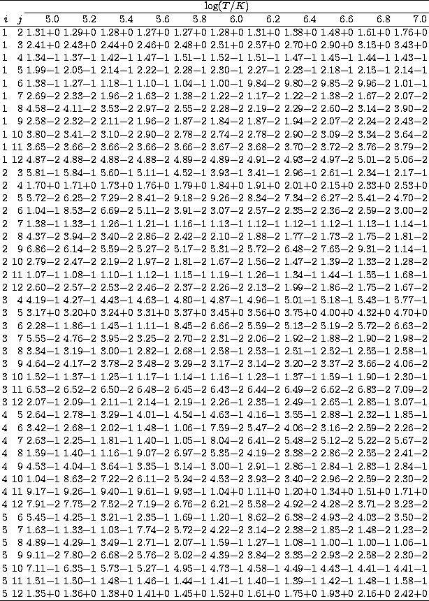
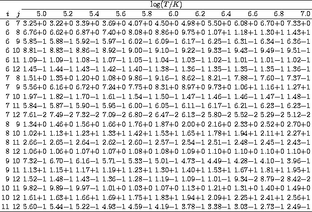
Table 6:
Present effective collision strength  for the
electron impact excitation of Fe XVI
for the
electron impact excitation of Fe XVI
|
|
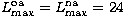
It is borne out by Table 5 that a ratio of two for the two
competing radii gives acceptable results. Convergence is excellent once the
first point of inflection of the partial waves appears at three times
the radius of the last point of inflection of the respective target
orbital. This condition is satisfied only at the first two energies for the
M-shell transitions. For transitions involving electrons with principal quantum
number  though this criterion is matched only at much higher
values of angular momentum l. In the present work we had to cut short the
expansion with respect to angular momenta at
though this criterion is matched only at much higher
values of angular momentum l. In the present work we had to cut short the
expansion with respect to angular momenta at
 , fine at 100Ryd
but somewhat tight when approaching 200Ryd (see Table 4).
It suffices for most transitions in the region
, fine at 100Ryd
but somewhat tight when approaching 200Ryd (see Table 4).
It suffices for most transitions in the region  Ryd,
although for one or two of the more difficult cases
incorrect high-energy tails required truncation at the breakdown point.
This situation is illustrated in Fig. 4 with the allowed transition
4pP
Ryd,
although for one or two of the more difficult cases
incorrect high-energy tails required truncation at the breakdown point.
This situation is illustrated in Fig. 4 with the allowed transition
4pP dD5/2, where the collision strength
is plotted using the scaling method of Burgess & Tully (1992).
It may be seen that the reduced collision strength at high energies correctly
approaches
dD5/2, where the collision strength
is plotted using the scaling method of Burgess & Tully (1992).
It may be seen that the reduced collision strength at high energies correctly
approaches  , but there is a point where this trend breaks
down. This problem can certainly be alleviated by increasing
, but there is a point where this trend breaks
down. This problem can certainly be alleviated by increasing
 -- at serious computational cost.
The slow partial wave convergence in some quadrupole transitions
is somewhat similar but not as acute; with a value of
-- at serious computational cost.
The slow partial wave convergence in some quadrupole transitions
is somewhat similar but not as acute; with a value of
 and a geometric series top-up such transitions
are accurately treated.
and a geometric series top-up such transitions
are accurately treated.
![\begin{figure}
\includegraphics []{8187f4.eps}\end{figure}](/articles/aas/full/1999/08/ds8187/Timg103.gif) |
Figure 4:
Reduced collision strength plotted as a function of the scaled
energy of Burgess & Tully (1992) (see Sect. 2) for the
 optically allowed
transition in Fe XVI showing the approach towards the high-energy
limit (filled circle). It may be seen the breakdown that takes place at
the higher energies due to an insufficiently high
(in this calculation optically allowed
transition in Fe XVI showing the approach towards the high-energy
limit (filled circle). It may be seen the breakdown that takes place at
the higher energies due to an insufficiently high
(in this calculation  ) ) |
The close-coupling calculation performed by Tayal (1994) for
Fe XVI is very similar to the present. A striking difference lies in his
treatment of the high partial waves, where for the optically allowed
transitions a cut-off value of  was adopted and a
geometric
series top-up was then implemented. For the forbidden transitions, on the other
hand, Tayal considered the total collision strengths converged
for
was adopted and a
geometric
series top-up was then implemented. For the forbidden transitions, on the other
hand, Tayal considered the total collision strengths converged
for  . By contrast we find in the present
work that reliable top-up procedures for some transitions,
specially within n=4 as discussed above,
could only be safely introduced at
much higher values of and
. By contrast we find in the present
work that reliable top-up procedures for some transitions,
specially within n=4 as discussed above,
could only be safely introduced at
much higher values of and  ,namely
  . The convergence of
some quadrupole transitions was found to be unusually slow. Tayal lists
collision strengths at 5 energies in the non-resonant region
(22.5, 36.0, 49.5, 67.5 and 90.0 Ryd)
and effective collision strengths in the electron-temperature
range
. The convergence of
some quadrupole transitions was found to be unusually slow. Tayal lists
collision strengths at 5 energies in the non-resonant region
(22.5, 36.0, 49.5, 67.5 and 90.0 Ryd)
and effective collision strengths in the electron-temperature
range  , thus
facilitating a thorough
comparison with present results. Cornille et al. (1997)
have computed collision strengths for the fine-structure transitions
with
, thus
facilitating a thorough
comparison with present results. Cornille et al. (1997)
have computed collision strengths for the fine-structure transitions
with  at 4 energy points in the non-resonant region (26, 50, 100 and
200 Ryd). A distorted wave method with TCC recoupling is used for
at 4 energy points in the non-resonant region (26, 50, 100 and
200 Ryd). A distorted wave method with TCC recoupling is used for
 at 26 and 50 Ryd, and
 at 100 and 200 Ryd. For
allowed transitions the Coulomb-Bethe top-up of Burgess & Shoerey
(1974) is used in the range
at 100 and 200 Ryd. For
allowed transitions the Coulomb-Bethe top-up of Burgess & Shoerey
(1974) is used in the range 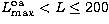 .The 3s-nd quadrupole transitions are topped-up for
 with the program NELMA
(Cornille
et al. 1994) based on a distorted wave approximation
without exchange.
with the program NELMA
(Cornille
et al. 1994) based on a distorted wave approximation
without exchange.
It is found that 85% of the collision strengths listed by
Tayal (1994)
agree with present results to within 10%. Large differences (up to 70%)
are found, however, for optically allowed transitions with
large collision strengths, in particular within the n=4 terms (e.g. 4s-4p,
4p-4d). This situation is clearly illustrated in Fig. 5 with the
 transition;
it may be seen that the reduced collision strengths by Tayal show an increasing
departure from the expected approach towards the high-energy limit. This
finding seems to indicate that his geometric series top-up for allowed
transitions can be unreliable at the high energies.
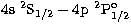
On the other hand only 76% of the collision strengths by
Cornille et al. (1997) are within the 10% level of agreement
with the present data. Larger differences are mainly found
towards the higher energies for the quadrupole transitions not arising from
the ground state (i.e. 3d-4s and n=n'=4) that have not been topped by
Cornille et al. beyond
transition;
it may be seen that the reduced collision strengths by Tayal show an increasing
departure from the expected approach towards the high-energy limit. This
finding seems to indicate that his geometric series top-up for allowed
transitions can be unreliable at the high energies.
On the other hand only 76% of the collision strengths by
Cornille et al. (1997) are within the 10% level of agreement
with the present data. Larger differences are mainly found
towards the higher energies for the quadrupole transitions not arising from
the ground state (i.e. 3d-4s and n=n'=4) that have not been topped by
Cornille et al. beyond  . In Fig. 6 we show
two cases where discrepancies at E=200 Ryd
are greater than 30%; in the transition
3dD3/2-4fF
. In Fig. 6 we show
two cases where discrepancies at E=200 Ryd
are greater than 30%; in the transition
3dD3/2-4fF it is seen that the agreement
is excellent except for the value at 200 Ryd, which is 50% higher; for
the 4sS
it is seen that the agreement
is excellent except for the value at 200 Ryd, which is 50% higher; for
the 4sS D3/2 the situation is similar,
but the high energy point is now 30% lower. The latter pattern is also found
in the following transitions: 4sSD5/2;
4pPpP and
4pPfF
D3/2 the situation is similar,
but the high energy point is now 30% lower. The latter pattern is also found
in the following transitions: 4sSD5/2;
4pPpP and
4pPfF .
.
![\begin{figure}
\includegraphics []{8187f5.eps}\end{figure}](/articles/aas/full/1999/08/ds8187/Timg117.gif) |
Figure 5:
Reduced collision strength for the
optically allowed
transition in Fe XVI. Solid curve: present results.
Crosses: Tayal
(1994). Filled squares: Cornille et al. (1997).
Filled circle: high-energy limit. The departure from the expected
approach to the high-energy limit observed in the values by Tayal are
believed to be due to an unreliable geometric series top-up |
![\begin{figure}
\includegraphics []{8187f6.eps}\end{figure}](/articles/aas/full/1999/08/ds8187/Timg119.gif) |
Figure 6:
Comparison of present collision strength (continuous curve)
with those computed by Cornille et al. (1997) (filled squares).
As shown for the transitions 4-12 (3dD3/2-4fF)and 6-9 (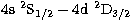 ),
the larger discrepancies are found for the high-energy point at 200 Ryd ),
the larger discrepancies are found for the high-energy point at 200 Ryd |
![\begin{figure}
\includegraphics []{8187f7.eps}\end{figure}](/articles/aas/full/1999/08/ds8187/Timg122.gif) |
Figure 7:
Comparison of present effective collision strength (circles)
with those computed by Tayal (1994) (filled squares).
Although good agreement is found
for most transitions, there are cases showing large discrepancies: for
instance transition 1-6
(3sS ) and
transition 4-5 ( ) and
transition 4-5 ( dD5/2) dD5/2) |
A comparison of the present effective collision strengths with those
tabulated by Tayal (1994) in the electron-temperature
range results in only
61% of the data agreeing to within 10% (82% to within 20%).
In Fig. 7 we show two transitions with significant differences:
3sS1/2-4sS1/2 (up to a factor of two) and
3dD (37%).
Regarding the former, the high values at the lower temperatures listed
by Tayal are due, in our opinion, to non-physical resonances caused by
the numerical instabilities discussed in connection with the use of
Option 1. The differences found in the transition within the 3d
(37%).
Regarding the former, the high values at the lower temperatures listed
by Tayal are due, in our opinion, to non-physical resonances caused by
the numerical instabilities discussed in connection with the use of
Option 1. The differences found in the transition within the 3d term
are more difficult to explain. Considerable differences are also found
for 3dD5/2-4sS1/2 and for transitions
with small (< 0.01) effective collision strengths.
term
are more difficult to explain. Considerable differences are also found
for 3dD5/2-4sS1/2 and for transitions
with small (< 0.01) effective collision strengths.
Up: Atomic data from the
Copyright The European Southern Observatory (ESO)
![\begin{figure}
\includegraphics []{8187f1.eps}\end{figure}](/articles/aas/full/1999/08/ds8187/img74.gif)
![\begin{figure}
\includegraphics []{8187f2.eps}\end{figure}](/articles/aas/full/1999/08/ds8187/img76.gif)
![\begin{figure}
\includegraphics []{8187f3.eps}\end{figure}](/articles/aas/full/1999/08/ds8187/img81.gif)
![\begin{tabular}
{r@{}c\vert cccccc}\hline &&&&&&&\\ [-1.5ex]
&&\multicolumn{6}{...
...2\\ & $LS$& 1.635 & 1.738 & 7.063 & 6.962 & 6.709 & 1.130\\ \hline\end{tabular}](/articles/aas/full/1999/08/ds8187/img91.gif)
![\begin{figure}
\includegraphics []{8187f4.eps}\end{figure}](/articles/aas/full/1999/08/ds8187/img103.gif)
![\begin{figure}
\includegraphics []{8187f5.eps}\end{figure}](/articles/aas/full/1999/08/ds8187/img117.gif)
![\begin{figure}
\includegraphics []{8187f6.eps}\end{figure}](/articles/aas/full/1999/08/ds8187/img119.gif)
![\begin{figure}
\includegraphics []{8187f7.eps}\end{figure}](/articles/aas/full/1999/08/ds8187/img122.gif)
![\begin{tabular}
{rc\vert ccc\vert ccc}\hline & &&& &&&\\ [-1.5ex]
\multicolumn{2...
... & 3.61\\ &$L+3$& 2.14 & 3.86 & 5.55 & 1.45 & 2.61 & 3.77\\ \hline\end{tabular}](/articles/aas/full/1999/08/ds8187/img87.gif)