In order to fulfile
condition 3 the NGSs are to be
located
within an angle ![]() from the optical axes, where
from the optical axes, where
![]() is the altitude of the highest relevant perturbing layer
(here and in the following we assume zenital or nearly zenital observations).
The area where the
is the altitude of the highest relevant perturbing layer
(here and in the following we assume zenital or nearly zenital observations).
The area where the ![]() NGSs stars are to be found is given,
expressed in square degrees, by the following:
NGSs stars are to be found is given,
expressed in square degrees, by the following:
 |
(7) |
In contrast, recall that the usable area
for classical NGS-based adaptive optics system is characterized by
a circular zone of radius ![]() , the so called isoplanatic patch,
of size
, the so called isoplanatic patch,
of size
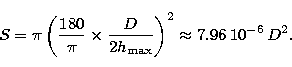
![]() .Assuming an average
.Assuming an average ![]() m
for both the SLC-N and HV-21 models (the two give respectively
m
for both the SLC-N and HV-21 models (the two give respectively
![]() m and
m and ![]() m for
m for ![]() ) a numerical estimation can
be made also:
) a numerical estimation can
be made also:
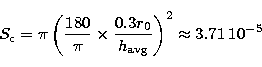 |
(8) |
where again the result is given in square degrees.
It should be pointed out in the latter that a single suitable NGS is to be found. However it is also remarkable that the points of the sky satisfying this last condition are biased by the presence of a relatively bright NGS within a small angle. Because of light scattering (or, at least, to the non negligible extension of the PSF) the sky background will be affected by some light negatively impacting extremely deep imaging. The classical sky coverage, or probability to find out a suitable NGS, is given by:
| (9) |
regardless of the telescope diameter D. Using a limiting magnitude
V0=13.0 as reported in Sect. 2, sky coverage of ![]() for
the Galactic poles (
for
the Galactic poles (![]() ) and
) and ![]() for the Galactic plane
(
for the Galactic plane
(![]() ) are retained.
) are retained.
In the tomographic case ![]() stars are to be found and the
probabilities composed in a multiplicative manner:
stars are to be found and the
probabilities composed in a multiplicative manner:
| (10) |
![\begin{figure}
\includegraphics [width=8.5cm]{ds1656f2.eps}\end{figure}](/articles/aas/full/1999/07/ds1656/img53.gif) |
Figure 2:
Sky coverage for various conditions vs. telescope diameter.
Continuous line is for V=12, |
Using the numerical estimation given in Eq. (7):
| (11) |
where one can note the dependence both from ![]() and D.
Inversion of Eq. (11) for D gives the following:
and D.
Inversion of Eq. (11) for D gives the following:
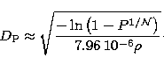 |
(12) |
Imposing P=0.50 or P=0.90 one can find the diameter where 50% and 90% of sky coverage is reached:
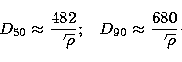 |
(13) |
Solving Eq. (12) for the classical NGS-based probabilities (P=0.02 for
![]() and P=0.002 for
and P=0.002 for ![]() ) one can find out also the critical
diameter
) one can find out also the critical
diameter ![]() as defined in the first section.
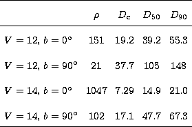
All these results are summarized in Table 2.
as defined in the first section.
All these results are summarized in Table 2.
 |
Equation (10) and followings do not impose any
particular geometry for the ![]() stars. Hence there is some chance
that these stars are placed on the sky in a way that avoids properly sensing
some portion of the highest layers. This problem is only mentioned here.
stars. Hence there is some chance
that these stars are placed on the sky in a way that avoids properly sensing
some portion of the highest layers. This problem is only mentioned here.
Copyright The European Southern Observatory (ESO)