The limiting magnitude for NGS-based adaptive optics system can be easily computed by both numerical and analytical formulations (Rigaut et al. 1997). Matching with experimental results is relatively satisfactory (Roddier 1998). In the LGS case the extension is straightforward only accepting conical anisoplanatism degradation and omitting the tip-tilt treatment. Few experimental results are available to confirm such results. To my knowledge there is no published result on noise propagation in tomographic wavefront sensing. It should be pointed out that in the modal formulation given by Ragazzoni et al. (1999) it would be easier to approach the problem in an analytical way because error-propagation in matrices involves straightforward matrices manipulation. A careful analysis and numerical confirmation, however, still requires a thorough discussion that is beyond the scope of this work.
At the current state of knowledge it is very hard to make a firm projection of the limiting magnitude for tomographic wavefront sensing. In this section I try to outline some considerations useful for giving a rough estimate of such limiting magnitude.
I assume that the following statements are true:
Let us suppose that, under some given conditions for the Fried parameter
r0, Greenwood frequency ![]() , overall quantum efficiency of the wavefront
sensing system q and its spectral bandwidth
, overall quantum efficiency of the wavefront
sensing system q and its spectral bandwidth ![]() expressed in nm,
a certain zonal error in the wavefront correction
expressed in nm,
a certain zonal error in the wavefront correction ![]() is obtained
when a star of magnitude V0 is used to close a classical adaptive
optics loop.
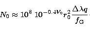
For each coherence zone (sized r0) of the collected wavefront and in a
single coherence time (of the order of
is obtained
when a star of magnitude V0 is used to close a classical adaptive
optics loop.
For each coherence zone (sized r0) of the collected wavefront and in a
single coherence time (of the order of ![]() ), the number of collected
photons N0 will be given by
(Zombeck 1990):
), the number of collected
photons N0 will be given by
(Zombeck 1990):
 |
(1) |
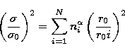
Each of these layers is numbered from 1 (the lowest) to ![]() (the
highest) and will be interested by an average number of NGSs given by ni.
For instance
(the
highest) and will be interested by an average number of NGSs given by ni.
For instance ![]() using the condition 1 and
using the condition 1 and ![]() using the condition 3. For each layer one can define a r0i
characteristic of the wavefront passing just through that portion of
turbulence.
using the condition 3. For each layer one can define a r0i
characteristic of the wavefront passing just through that portion of
turbulence.
Supposing the use of a
star of magnitude V0 to sense directly just the i-th single layer a
number of photons given by:
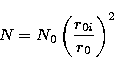 |
(2) |
 |
(3) |
 |
(4) |
In order to reach
with
the tomographic approach the same zonal error
as
the classical
single guide star approach,
a limiting magnitude for each of the ![]() NGS (the
condition 2 is used here) of:
NGS (the
condition 2 is used here) of:
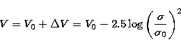 |
(5) |
 |
(6) |
Conservatively we assume in the following ![]() , that is V=12.0
or V=14.0
as extrema of limiting magnitudes for the NGSs to be used in the tomographic
approach.
While no attempt is made to use many more fainter NGSs to mimic fewer brighter NGSs
(an approach that could widen the practicability of the proposed approach)
the approximate and tentative nature of these calculations must be reiterated.
Also, it
should
be pointed out that essentially no literature is available on possible
techniques for efficient wavefront sensing and correction in the tomographic
mode and there is no evidence that straightforward sensing with classical
wavefront sensor of each star to be coupled together in a dedicated
wavefront computer represent the ultimate achievable performance.
Moreover
I have
not speculated on the possibility
of using
NGSs to
directly retrieve
tomographic information as suggested for instance by
Ribak (1995).
, that is V=12.0
or V=14.0
as extrema of limiting magnitudes for the NGSs to be used in the tomographic
approach.
While no attempt is made to use many more fainter NGSs to mimic fewer brighter NGSs
(an approach that could widen the practicability of the proposed approach)
the approximate and tentative nature of these calculations must be reiterated.
Also, it
should
be pointed out that essentially no literature is available on possible
techniques for efficient wavefront sensing and correction in the tomographic
mode and there is no evidence that straightforward sensing with classical
wavefront sensor of each star to be coupled together in a dedicated
wavefront computer represent the ultimate achievable performance.
Moreover
I have
not speculated on the possibility
of using
NGSs to
directly retrieve
tomographic information as suggested for instance by
Ribak (1995).
 |
Copyright The European Southern Observatory (ESO)