3 Simulation study

  The goal of this simulation study is to assess the quality of the approximation under various orbital and pulsation models. We consider a simplified model with at most two pulsational modes:  

$$\begin{array} {l} v_{t\lambda}=\beta(t)+\alpha_1\sin(\omega_... ...pha_2\sin(\omega_2t+\phi_2) +\varepsilon_{t\lambda}.\end{array}$$ (14)

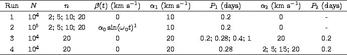
We performed four small simulation runs. Each time a beat period is covered with a grid of equally spaced points and for each point (14) is calculated, where the error term $\varepsilon_{t\lambda}$ is generated from a standard normal distribution. Then, we slide a window through the beat period and for the set of observations within a window, a sinusoidal approximation is calculated. From this approximation, the amplitude is retained. From these amplitudes, $\mu$ and $\tau^2$ can be estimated and hence our proposed expression for the standard deviation (13) can be computed. The purpose of this study is to compare this with the "correct'' value, which is determined as the sample standard deviation of $v_{t\lambda}-\beta(t)$ in (14). Rewrite $\omega_i=2\pi/P_i$, where P_i is the period in days. Apart from the parameters in (14) we need to specify the number N of equally spaced times t under consideration. In addition, the number of replications n at each time needs to be specified. The settings are displayed in Table 1. All phases are chosen $\phi_1\equiv 0$.

 

Table 1: Simulation settings

 

¹: Here, $\alpha_0=50$ (km s^-1) and d₀=5;50;100 (days).

Once we can conclude that the results are acceptable, it follows that (12) can be trusted since the only difference between (12) and (13) is that (12) further corrects for the fact that several replicates are taken at time t. In the simulation settings considered here, the discrepancy between (13) and (12) is of the order of 0.5% of (13).

In the first and the second simulation, there is only one pulsational mode and therefore the observed amplitude is constant over time, implying that $\tau^2\equiv 0$. The second simulation allows for a non-constant $\beta(t)$which, for simplicity, is assumed to be of sinusoidal form as well. In order to adequately cover the rapidly varying wave throughout the beat period, the number of times N was increased by a factor 10. In both simulations, the true standard deviation is about 7.14km s^-1. We observe a relative error between (13) and the true value smaller than 0.23% in the first simulation and smaller than 0.15% in the second simulation. This confirms the correctness of the formula (13).

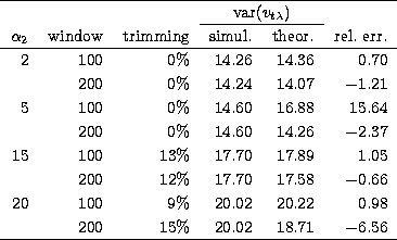
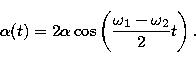
The third simulation studies the particular case of two pulsational modes with $\alpha_1=\alpha_2=\alpha$, implying that

$$\alpha\sin(\omega_1t) +\alpha\sin(\omega_2t) =\alpha(t)\sin(\omega t)$$

with $\omega$ the average of $\omega_1$ and $\omega_2$ and  

$$\alpha(t)=2\alpha\cos\left( \frac{\omega_1-\omega_2}{2}t \right).$$ (15)

Therefore, (15) can be used to determine $\mu^2+\tau^2$. The true standard deviations range between 20km s^-1 and 30km s^-1 and the largest discrepancy between our formula and the correct value is 0.17%.

In practice, formula (15) will not be available to determine the statistical properties of the varying amplitude. Rather, it must be estimated from a set of data. This is classically done using either Fourier transforms or minimization in the least squares sense (Bloomfield 1976) which is a special case of a statistical optimization method known as profile likelihood (Welsh 1996). We used the second method in the fourth simulation, which also enables us to cover the situation $\alpha_1\ne \alpha_2$. Practically, we fitted a function

$$\delta+\alpha\sin(\omega t+\phi)$$

to a window of the data generated under one of the settings of the fourth study. The window consisted either of 100 or of 200 successive points (out of 1000). Windows were then shifted with increments of 10, giving us 90 or 80 different values. In some regions, and for amplitudes that are either equal or similar ($\alpha_2=15,20$), the fit was difficult and yielded implausible values for $\alpha$. Therefore, we applied trimming, i.e., we discarded all values $\alpha$ larger than 50. The results are presented in Table 2.

 

Table 2: Results for simulation study 4

 

Observe that there is some difficulty to recover the correct simulated values when $\alpha_1=20$ km s^-1 and $\alpha_2$ lie fairly close to each other. In those cases, some trimming was necessary. In addition, there appears to be some impact from the choice of window.