Up: Corrections and new developments
In this chapter our aim is to calculate the coefficients of the nutation related
to the spin-orbit effect with a better accuracy than previously
(Kinoshita & Souchay 1990),
and by picking up all the coefficients larger than  . Kubo (1982) showed that the Earth flattening is perturbing the orbital motion of the Moon, and
this perturbation itself is modifying the motion of nutation of the Earth.
The determination of the perturbation due to this reciprocical influence can be tackled
when considering the global Earth-Moon system, not the system formed by the Earth itself,
as it is the case in classical theories not involving the Hamiltonian (Woolard 1953).
Kinoshita & Souchay (1990) included this effect in their second-order calculations involving the
Delaunay canonical angular variables l', g' and h', and action variables L', G'
and H'. l' is the mean anomaly of the Moon, g' is the argument of the perigee and h'
is the longitude of the node, with respect to the ecliptic. The action variables have the
following expressions:
. Kubo (1982) showed that the Earth flattening is perturbing the orbital motion of the Moon, and
this perturbation itself is modifying the motion of nutation of the Earth.
The determination of the perturbation due to this reciprocical influence can be tackled
when considering the global Earth-Moon system, not the system formed by the Earth itself,
as it is the case in classical theories not involving the Hamiltonian (Woolard 1953).
Kinoshita & Souchay (1990) included this effect in their second-order calculations involving the
Delaunay canonical angular variables l', g' and h', and action variables L', G'
and H'. l' is the mean anomaly of the Moon, g' is the argument of the perigee and h'
is the longitude of the node, with respect to the ecliptic. The action variables have the
following expressions:
| ![\begin{displaymath}
L' = \Bigl[ {M_{\rm E} M_{\rm M}
\over M_{\rm E} + M_{\rm M} } \Bigr] \times \sqrt{\mu a_{\rm M}} \end{displaymath}](/articles/aas/full/1999/04/ds7187/img93.gif) |
(17.1) |
|  |
(17.2) |
|  |
(17.3) |
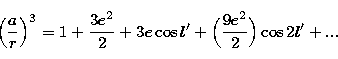
For the calculations to be achieved properly, the spherical coordinates
 ,
,  and
and  must be replaced by their expressions in function
of the canonical variables in the Eq. (3) giving the expression of
the potential. is related to the canonical variables H'
and G' by the intermediary
of the
must be replaced by their expressions in function
of the canonical variables in the Eq. (3) giving the expression of
the potential. is related to the canonical variables H'
and G' by the intermediary
of the  variable which represents the inclination of the Moon'sorbit on the ecliptic.
We have:
variable which represents the inclination of the Moon'sorbit on the ecliptic.
We have:
|  |
(18) |
Moreover is the sum of the three angular variables:
| 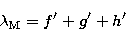 |
(19) |
f' being the true anomaly of the Moon. For reasons of commodity, the indices
M will be omitted, in the following, concerning the variables  , and
, and  .By substituing the values of
  and in equation (3) we find
the following development for
and in equation (3) we find
the following development for  , which is the expression of the lunar
potential at the first order:
, which is the expression of the lunar
potential at the first order:
|  |
|
| |
| |
| |
| |
| |
| |
| (20) |
Where  and f' are themselves a function of the
mean anomaly of the Moon l' and of the eccentricity :
and f' are themselves a function of the
mean anomaly of the Moon l' and of the eccentricity :
|  |
(21) |
| 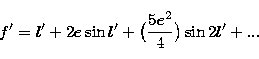 |
(22) |
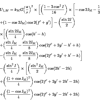
The second-order potential  characterizing the spin-orbit coupling
effect has the same expression as in (1), but by substituting the
Delaunay's variables h' and H' to the Andoyer's variables h and H:
characterizing the spin-orbit coupling
effect has the same expression as in (1), but by substituting the
Delaunay's variables h' and H' to the Andoyer's variables h and H:
| ![\begin{eqnarray}
&&W_2^{\rm cpl.} {=} \Biggl( {1 \over 2} \int\Bigl[ {\partial (...
...tial (W_{1}) \over \partial l'}\Bigr] {\rm d}t \Biggr)_{\rm per}.n\end{eqnarray}](/articles/aas/full/1999/04/ds7187/img107.gif) |
|
| |
| (23) |
Using the Eqs. (17.1-3) we obtain the derivative of a given function with respect
to L',G' and H' starting from its derivatives with respect to a,e and :
| ![\begin{displaymath}
{\partial [...] \over \partial L'} = {2 L' \over \mu}
\time...
... - e^{2}) \over e L'}
\times{\partial [...] \over \partial e} \end{displaymath}](/articles/aas/full/1999/04/ds7187/img108.gif) |
(24) |
| ![\begin{displaymath}
{\partial [...] \over \partial G'} = {-\sqrt{1 - e^{2}} \ove...
...ot I_{\rm M} \over G'}{\partial [...] \over \partial I_{\rm M}}\end{displaymath}](/articles/aas/full/1999/04/ds7187/img109.gif) |
(25) |
| ![\begin{displaymath}
{\partial [...] \over \partial H'} = - {1 \over G' \sin I_{\rm M}}
\times{\partial [...] \over \partial I_{\rm M}} \cdot \end{displaymath}](/articles/aas/full/1999/04/ds7187/img110.gif) |
(26) |
Because of the expected relative smallness of the nutation coefficients coming from the
spin-orbit coupling effect, we can initially restrict ourselves to the leading terms of the
potential as given by (20). Practically we can keep the components which remain
large enough after integration, that is to say those
whose the product of the amplitude and of the inverse of the frequency are the
largest ones. As a result of the procedure, we retain in fact 6 terms with the
argument  ,
,  ,
,  ,
,  ,
,  and
and
 ( is the mean anomaly of the Moon, the mean
longitude of the node, and F is given by:
( is the mean anomaly of the Moon, the mean
longitude of the node, and F is given by:  , where
  is
the mean longitude of the Moon).
is
the mean longitude of the Moon).
To have an idea of their respective values, we can refer to the tables of the potential
listed in Kinoshita (1977).
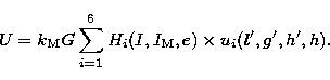
Each of these components can be represented as a product 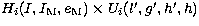 . This makes the calculations easier for Hi (i=1,6) depends
only on the canonical action variables, whereas Ui(l',g',h',h) (i=1,6)
only depends on the angle canonical variables. We can thus adopt for the potential the
following development:
. This makes the calculations easier for Hi (i=1,6) depends
only on the canonical action variables, whereas Ui(l',g',h',h) (i=1,6)
only depends on the angle canonical variables. We can thus adopt for the potential the
following development:
|  |
(27) |
With:
| 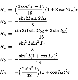 |
|
| |
| |
| |
| |
| (28) |
| 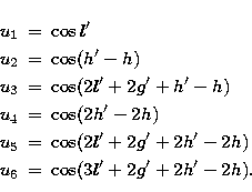 |
|
| |
| |
| |
| |
| (29) |
By combining the Eqs. (23), (24), (25) and (26) with the help of the form
given by (27), (28) and (29), then we can get a rather straightforward final expression
for the second-order determing function related to the coupling
effect that we are dealing with here, that is to say:
|  |
|
| |
| |
| |
| |
| (30) |
With the following developments for Ai:
| ![\begin{eqnarray}
A_{1} &=& \sum_{i=1}^{6} \sum_{j=1}^{6} H_{i} {\partial H_{j} \...
...
- w_{j} \Bigl( {\partial u_{i} \over \partial l'} \Bigr) \Bigr] \end{eqnarray}](/articles/aas/full/1999/04/ds7187/img122.gif) |
|
| |
| |
| |
| (31) |
where wi (i=1,6) is obtained with a simple integration of ui:
| 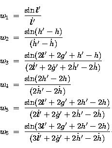 |
|
| |
| |
| |
| |
| (32) |
Then the nutations in longitude  and
and
 coming from are
given by:
coming from are
given by:
| 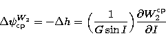 |
(33) |
and:
| ![\begin{displaymath}
\Delta \varepsilon_{\rm cp}^{W_{2}} = -\Delta I =
- \Bigl[ {...
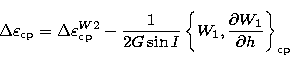
...\sin I} \Bigr] {\partial W_{2}^{\rm cp} \over \partial h}\cdot \end{displaymath}](/articles/aas/full/1999/04/ds7187/img127.gif) |
(34) |
The expressions  and
and  which characterize the
total spin-orbit coupling effect are then given by (Kinoshita & Souchay 1990):
which characterize the
total spin-orbit coupling effect are then given by (Kinoshita & Souchay 1990):
|  |
(35.1) |
|  |
(35.2) |
we insist on the fact that as long as we dealt with crossed-nutation, for instance
in (14.1) and (14.2) the Poisson brackets  were calculated with respect
to the Andoyer canonical variables l, g, and h. In this section which concerns the
coupling effect, the Poisson brackets
were calculated with respect
to the Andoyer canonical variables l, g, and h. In this section which concerns the
coupling effect, the Poisson brackets  are calculated with respect
to the Delaunay canonical variables l', g' and h'. It is also important to keep in mind that
the derivatives with respect to a in the ui's and the wi's (where a is
the
semi-major axis for the keplerian motion) is not 0, for the coefficient
are calculated with respect
to the Delaunay canonical variables l', g' and h'. It is also important to keep in mind that
the derivatives with respect to a in the ui's and the wi's (where a is
the
semi-major axis for the keplerian motion) is not 0, for the coefficient  in the expression of the potential
  in Eq. (20) contains (a3)-1
at the denominator. Then these derivatives have to be taken into account when calculating
the derivatives with respect to L', according to (24). This explains the presence of
the coefficient A5 in (30) and (31).
in Eq. (20) contains (a3)-1
at the denominator. Then these derivatives have to be taken into account when calculating
the derivatives with respect to L', according to (24). This explains the presence of
the coefficient A5 in (30) and (31).
Let us now introduce the following quantities:
and

that is to say:
|  |
(36.1) |
|  |
(36.2) |
|  |
(36.3) |
|  |
(36.4) |
|  |
(36.5) |
|  |
(36.6) |
and:
|  |
(37.2) |
|  |
(37.3) |
|  |
(37.4) |
|  |
(37.5) |
|  |
(37.6) |
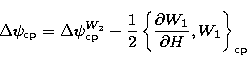
Then the complementary term of the nutation in longitude, which corresponds to the
part inside the Poisson brackets in (35.1), is given by:
| ![\begin{eqnarray}
&&\Delta \psi_{\rm cp}^{\rm comp} =
- { 1 \over 2} \left\lbrac...
...r]
\times \left({\partial w_{i} \over \partial l'}\right) w_{j} .\end{eqnarray}](/articles/aas/full/1999/04/ds7187/img148.gif) |
|
| |
| |
| |
| |
| (38) |
Table 2:
List of the coefficients of rigid Earth
nutation coming from the spin-orbit coupling effects
 |
And the complementary term of the nutation in obliquity in (28.2) can be expressed in a
similar way by:
| ![\begin{eqnarray}
&&\Delta \varepsilon_{\rm cp}^{\rm comp} =
\left[{1 \over 2G\s...
...\partial l'} -
z_{j}{ \partial w_{i} \over \partial l'} \right].\end{eqnarray}](/articles/aas/full/1999/04/ds7187/img150.gif) |
|
| |
| |
| |
| |
| |
| |
| |
| (39) |
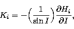
For our present computations, the parameter  is necessary. It
represents the ratio of the spin angular-momentum of the Earth to
the orbital angular momentum of the Moon, and can be expressed as follows:
is necessary. It
represents the ratio of the spin angular-momentum of the Earth to
the orbital angular momentum of the Moon, and can be expressed as follows:
|  |
(40) |
Its value is:  .
.
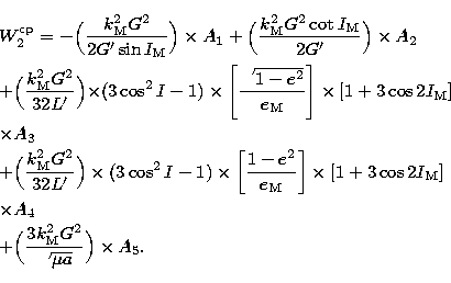
The results related to the spin-orbit effect as studied here are listed in
Table 2. We can remark that the number of coefficients down to is
much smaller than what was found in the previous section for the
crossed-nutation contribution. Also we can remark that the leading coefficient is by far
the 18.6y component, both in longitude and in obliquity, with respective
in-phase values of  and
and  .The analytical expressions for these two leading terms are given by the rather cumbersome
following formulas:
.The analytical expressions for these two leading terms are given by the rather cumbersome
following formulas:
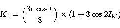
| 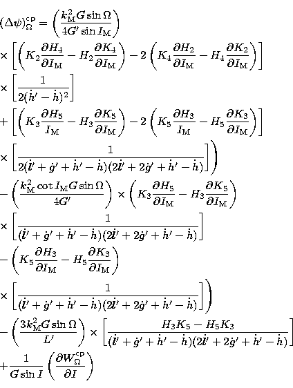 |
|
| |
| |
| |
| |
| |
| |
| |
| |
| |
| (41) |
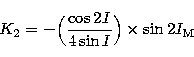
and:
| 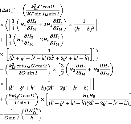 |
|
| |
| |
| |
| |
| |
| |
| (42) |
where  itself is expressed as a function of
the Hi:
itself is expressed as a function of
the Hi:
| ![\begin{eqnarray}
&&W_{\Omega}^{\rm cp} = \left(
\frac{k_{\rm M}^{2} G^{2} \sin ...
... 2\dot g' + \dot h' - \dot h)(\dot h' - \dot h)} \right] \right)
,\end{eqnarray}](/articles/aas/full/1999/04/ds7187/img159.gif) |
|
| |
| |
| |
| |
| |
| |
| (43) |
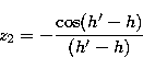
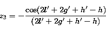
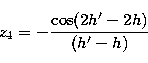
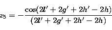
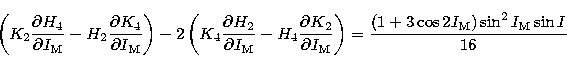
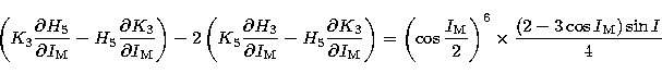
with:  . In Eqs. (40), (41), and (42), we use the following
substitutions, with the help of (27.1-6) and (36.1-6):
. In Eqs. (40), (41), and (42), we use the following
substitutions, with the help of (27.1-6) and (36.1-6):
|  |
(44.1) |
|  |
(44.2) |
|  |
(44.3) |
|  |
(44.4) |
|  |
(44.5) |
|  |
(44.6) |
|  |
(44.7) |
Remark that the second largest component in Table 2 with argument and
with period 13.66d (fortnightly), was not found in previous calculations
(Kinoshita & Souchay 1990), because of their incompleteness.
On the opposite the two terms of argument and  were
already present in these calculations. An important part of the
present ones were carried out by the help of Mathematica, a precious tool to
compute formal analytical expressions.
were
already present in these calculations. An important part of the
present ones were carried out by the help of Mathematica, a precious tool to
compute formal analytical expressions.
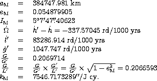
The numerical values of the constant terms used in the present section
are taken from ELP2000 (Chapront-Touzé & Chapront 1988) except for
(Souchay & Kinoshita 1996) and the ratio calculated
above. They are given as follows:
Up: Corrections and new developments
Copyright The European Southern Observatory (ESO)