5 Streaming

  The sub-sample with observed radial velocities is incomplete and contains biases since the stars are not observed at random. To keep the benefits of the sample completeness, a statistical convergent point method is developed to analyze all the stars (Sect. 5.1). However, this method creates spurious members among detected streams with wavelet analysis, Sect. 5.2.1 describe the procedure to handle their proportion. Moreover the fraction of field stars detected as stream members is also evaluated through the procedure in Sect. 5.2.2.

5.1 Recovering 3-D velocities from proper motions: A convergent point method

 U, V and W velocities are reconstructed from Hipparcos tangential velocities by a convergent point method for stars which belong to streams. All pairs of stars are considered; each pair gives a possible convergent point (assuming that both stars move exactly parallel) and the radial velocity is inferred for each component. Then fully reconstructed velocities of the two stars, V₁ and V₂, are considered only if $\mid V_{1}-V_{2} \mid$ does not exceed a fixed selection criterion. This pre-selection of reconstructed velocities eliminates most of false reconstructions. In the following, the criterion is fixed to 0.5 km s^-1.

  

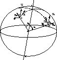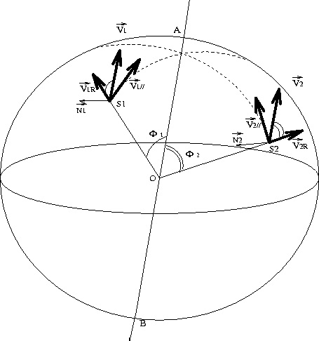
Figure 11: Implementation of the convergent point method. $\vec{V_{1\parallel}}$,$\vec{V_{2\parallel}}$ are the tangential velocities measured by Hipparcos for two stars. $\vec{V_{1R}}$, $\vec{V_{2R}}$, are deduced radial velocities assuming that stars S1 and S2 belong to the same stream

The convergent point algorithm (see Fig. 11) follows the steps:

1.

keep a pair of stars (S₁,S2),

2.

define vectors $\vec{N_{1}}$ and $\vec{N_{2}}$ which are perpendicular respectively to the plane ($\vec{OS_{1}}$,$\vec{V_{1\parallel}}$) and ($\vec{OS_{2}}$,$\vec{V_{2\parallel}}$),

3.

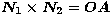obtain $\vec{N_{1}} \times \vec{N_{2}} = \vec{OA}$ which is the direction of the hypothetical convergent point A,

4.

test the coherence of this direction with both tangential velocities: if sgn($\vec{OA} \cdot \vec{V_{1\parallel}}$) $\neq$ sgn($\vec{OA} \cdot \vec{V_{2\parallel}}$), it is not a convergent point. Go to 1,

5.

calculate angles between star directions and the convergent point: $\Phi_{1}$=($\widehat{\vec{OS_{1}},\vec{OA}}$) and $\Phi_{2}$=($\widehat{\vec{OS_{2}},\vec{OA}}$),

6.

infer moduli and signs of radial velocities:

$$\begin{eqnarray} V_{\rm R}=\frac{V_{\parallel}}{\tan\Phi}&{\rm if}&\Phi < \frac{... ...-\pi)}&{\rm if}&\Phi \gt \frac{\pi}{2} \ {\rm and} \ \Phi \neq \pi\end{eqnarray}$$ (10)

7.

calculate space velocities V₁ and V₂ which vectors are strictly parallels by construction

$$V = \sqrt{V_{\parallel}^{2}+V_{\rm R}^{2}}$$ (11)

8.

test agreement between V₁ and V₂ within tolerance $\eta$
$\mid V_{1} - V_{2} \mid \leq \eta$ with fixed $\eta$ = 0.5 km s^-1.

Following this process, a large number of may-be velocities are calculated. Several definitions of each star velocity are obtained. All are distributed along a line in the 3D velocity space, part of them being spurious. Real streams produce over-density clumps formed by line intersections. The wavelet analysis detects such clumps in the (U, V, W) distributions. The detection sensitivity is tested numerically by simulating a variety of stream amplitudes and velocity dispersions over a velocity ellipsoid background. Simulations show that our wavelet analysis implementation is able to discriminate streams formed by at least 16 stars non-spatially localized and moving together with a typical velocity dispersion of 2 km s^-1 in a velocity background matching the sample's one. The scale at which the stream velocity is detected is a measure of the stream velocity dispersion. A more accurate knowledge of this parameter is obtained after the full identification of the members (see Sect. 5.3).

Velocities of open cluster stars are poorly reconstructed by this method because their members are spatially close. For such stars, even a small internal velocity dispersion results a poor determination of the convergent point. For this reason, we have removed stars belonging to the 6 main identified space concentrations (Hyades OCl, Coma Berenices OCl, Ursa Major OCl and Bootes 1, Pegasus 1, Pegasus 2 groups) found in the previous spatial analysis. Eventually, the reconstruction of the velocity field is performed with 2910 stars.

Reconstructed (U, V, W) distributions are given in an orthonormal frame centred in the Sun velocity in the range [-50, 50] km s^-1 on each component. The wavelet analysis is performed on five scales: 3.2, 5.5, 8.6, 14.9 and 27.3 km s^-1. In the following, the analysis focuses on the first three scales revealing the stream-like structures because larger ones reach the typical size of the velocity ellipsoid. Once the segmentation procedure is achieved, stars belonging to velocity clumps are identify. The set of velocity definitions of a star may cross two velocity clumps. In this case, the star is associated with the clump in which it appears most frequently.

5.2 Cleaning stream statistics

 

5.2.1 Estimating the fraction of spurious members in velocity clumps

 Despite the pre-selection of reconstructed velocities ($\mid V_{1} - V_{2} \mid \leq \eta$)some spurious velocities are still present in the field. For this reason, real velocity clumps do include some proportion of spurious members generated by the convergent point method. Estimating the proportion of spurious members in each velocity clump is essential and is done by comparing the mean of reconstructed radial velocities of each star with its observed radial velocity whenever this data is available (1362 among 2910 stars). For each star in a stream, the following procedure is adopted:

1.

Only radial velocities reconstructed with other suspected members of the same stream are considered.

2.

Mean $\overline{V_{R_{\rm rec.}}}$ and dispersion $\sigma_{V_{R_{\rm rec.}}}$ of the reconstructed radial velocity distribution are calculated (Fig. 12).

  

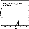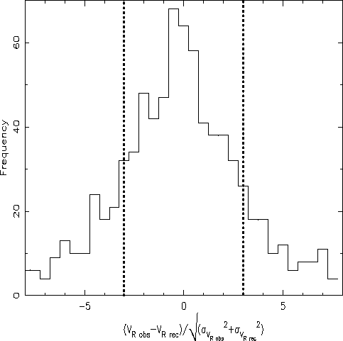
Figure 12: Example of $V_{R_{\rm rec.}}$ distribution for one star suspected to be member of a stream and its observed radial velocity (dot dashed line)

3.

The star is confirmed to belong to the stream when the normalized residual

$$R_{N}=\frac{\mid V_{R_{\rm obs.}}-\overline{V}_{R_{\rm rec.}... ..._{R_{\rm rec.}}}^{2}+ \sigma_{V_{R_{\rm obs.}}}^{2}}} \nonumber$$

doesn't exceed a value $\kappa$. Residuals take into account errors $\sigma_{V_{R_{\rm obs.}}}$ on the observed radial velocities given in the Hipparcos Input Catalogue. These errors are classified into 4 main values: 0.5, 1.2, 2.5, 5 km s^-1. The threshold $\kappa$ is fixed empirically on the basis of the normalized residual histogram of all suspected stream members with observed radial velocities (Fig. 13) at scale 2. It is set to $\mid\kappa\mid$ = 3 in order to keep the bulk of the central peak. The results of this paper are robust to any reasonable change of $\mid\kappa\mid$ between 2.5 and 4.

  

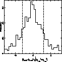Figure 13: Distribution of weighted radial velocity deviates (normalized residual) for all suspected stream members with observed radial velocity at scale 2. Dashed line delimits the area of high probability of false detection

  

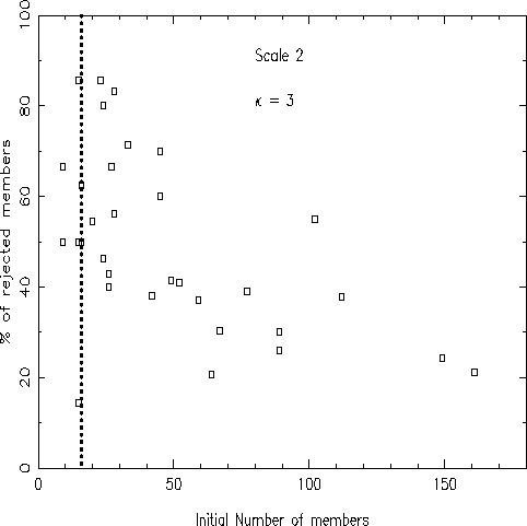
Figure 14: Proportion of rejected members for all the detected velocity clumps at scale 2 by the selection on observed radial velocity function of the initial number of members. Dashed line indicates the minimum number of stream members requires to detect streams in simulations

 

Figure 15: Hyades Scl. Thresholded wavelet coefficient isocontours at W=-2.4 km s^-1 of the velocity field at scale 3 (top left) and scale 2 (top right). This slice in wavelet coefficients at scale 2 reveals two of the three clumps composing the whole supercluster. Age distributions of the whole group (stream 3-10 in Table 2) at third scale (middle left) and of the first sub-stream (stream 2-10 in Table 3) at second scale (middle right). Age distributions of the two last sub-streams (stream 2-18 and 2-25 in Table 3) discovered at scale 2 (bottom)  

Noise estimations in each velocity clump for the three first scales (provided that they have at least 3 stars with observed V_R), following the procedure quoted above, are shown in Fig. 14. There are two regimes in these noise estimations: streams with more than 50 initial suspected members ($N_{\rm init}$) which have a contamination by spurious members around 30$\%$; streams with less than 50 initial suspected members which may have a contamination up to 85$\%$. In this extreme case, should we say that these streams are false detection? Not necessarily, because our denoising method is too drastic towards small streams. Indeed, in those, each star has very few reconstructions of its radial velocity with the other members of the

same stream. The dispersion of the reconstructed $V_{\rm R}$ distribution is necessarily small, implying an important normalized residual. Then, the star is often rejected. If we refer to our previous simulations there is a high probability that under 16 initial members, streams are false detection.

At the end of this selection we obtain the number of confirmed members among stars with observed V_R in each stream for the three first scales (column $N_{\rm sel}$ in Tables 2, 3 and 4) and their sum (line Total 2 in column $N_{\rm sel}$).

  

Table 2: Main characteristics of detected streams at scale 3 with filter size of 8.6 km s^-1 ($\overline{\sigma}_{\rm stream}\sim$ 6.3 km s^-1). $\overline{\bf U} \pm \sigma_{u}$, $\overline{\bf V}\pm \sigma_{v}$ and $\overline {\bf W} \pm \sigma_{w}$ are the mean velocity components and their dispersions calculated, after selection on $V_{\rm R}$, with the true radial velocity data - $N_{\rm init}$ is the initial number of stars belonging to the structure - $N_{V_{\rm R}}$ is the number of stars with observed radial velocity - $N_{\rm sel}$ is the number of stars among $N_{V\rm _r}$ after selection 5.2.1. The selection has not been done in case where there is less than 3 observed radial velocities. In this last case an d also when none of the stars are selected we do not present the line in the table. However the same stream identifiers are conserved: the first digit is the scale followed by the stream number. Column $\%_{\rm field}$ is the percentage of field st ars estimated in each structure with the procedure 5.2.2. Cross-identification is done with Eggen's superclusters (SCl) and open cluster (OCl) data from Paloùs and Eggen (in Gomez et al. 1990) (see Table 5) - Total 1 gives the s um of suspected stream members (Col. $N_{\rm init}$) and the sum of observed V_R among them (Col. $N_{V_{\rm R}}$) - Total 2 gives the sum of all confirmed stream stars among available observed radial velocities (Col. $N_{\rm sel}$) - Total 3 is the sum of all expected stream members in each stream (Col. $N_{\rm init}$) taking into account the confirmed/suspected ratio obtained in each stream - Total 4 gives the inferred fraction of stars in stream in the full sample of 2910 stars (Col. $N_{\rm init}$). Total 5 is the fraction of stars in stream corrected for field contamination (Col. $N_{\rm init}$)

  

Table 3: Main characteristics of detected velocity structures at scale 2 with filter size of 5.5 km s^-1 ($\overline{\sigma}_{\rm stream}\sim$ 3.8 km s^-1). Legend is the same as Table 2

  

Table 4: Main characteristics of detected velocity structures at scale 1 with typical size of 3.2 km s^-1 ($\overline{\sigma}_{\rm stream}\sim$ 2.4 km s^-1). Legend is the same as Table 2

  

Table 5: Cross-identification data for known kinematical groups: Open clusters (OCl) and Superclusters (SCl)

5.2.2 Estimating the proportion of field stars in velocity clumps

 The fraction of a smooth distribution filling the velocity ellipsoid of our complete sample, expected inside the velocity volume spanned by the 6 superclusters described bellow, range between 2$\%$ and 4$\%$ depending on the position of the structure with respect to the distribution centroid. Adding up these contributions, 19.2$\%$ of field stars should be expected to fill the total volume occupied by superclusters with pure random coincidence. This is about $20-30\%$ of the stars detected as supercluster members at scale 3. However, streams with smaller velocity dispersions (scales 1 and 2) are not significantly affected by this background. Proportions of field stars for the largest structures found at scale 3 are given in 2 at column $\%_{\rm field}$ while it is neglected for the remaining streams.

5.3 Stream phenomenology

 Tables 2, 3 and 4 give mean velocities, velocity dispersions and numbers of stars remaining after correction of spurious members (procedure 5.2.1) and field stars (procedure 5.2.2) for streams at respectively scale 3, 2 and 1. Each stream has $N_{V_{\rm r}}$ observed radial velocity members. Out of the $N_{V_{\rm r}}$ stars with radial velocities among suspected stream members, only $N_{\rm sel}$ get confirmed by procedure 5.2.1. So the ratio $N_{\rm sel}$/$N_{V_{\rm r}}$ is an estimate of the confirmed/suspected ratio in each stream. Applying this ratio to $N_{\rm init}$ (total stream member candidates) we get the expected number of real stream members in each stream, and the total number of stream members in the sample (Total 3). The percentage of stars in streams in the total sample follows ( Total 4). The correction for the uniform background contribution is negligible at scales 1 and 2; it is significant at scale 3 where the fraction of stars in streams drops from 63.0$\%$ to 46.4$\%$. In the case of large velocity dispersion structures at scale 3 proportions of field stars is also given in column $\%_{\rm field}$ and the percentage of remaining stream stars is done in column $N_{\rm init}$ line Total 5.

  

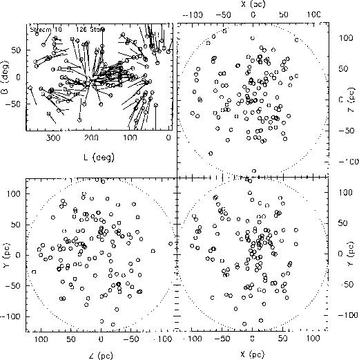
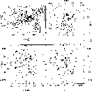Figure 16: Space distribution of Hyades SCl from the $V_{\rm R}$ selected sub-sample at scale 3 (stream 3-10 in Table 2)

  

Figure 17: Sirius Scl. Thresholded wavelet coefficient isocontours at W=-10.1 km s^-1 of the velocity field at scale 3 (top left) and scale 2 (top right). At scale 2, Sirius SCl is composed of 2 main streams (stream 2-37 and 2-41 in Table 3). The 2$^{\rm nd}$ is shown on this W slice of wavelet coefficients. Age distributions of the whole Sirius SCl at third scale (middle left) and stream 2-37 at second scale (middle right). Age distribution s of stream 2-41 at scale 2 (bottom left) and stream 1-56 (in Table 4) at scale 1 (bottom right). This latest figure (highest resolution) shows that separating oldest populations is out of reach

5.3.1 Particulars on superclusters

 Streams appearing at scale 3 ($\overline{\sigma}_{\rm stream}\sim$ 6.3 km s^-1) correspond to the so-called Eggen superclusters. Four already known such structures are found: the Pleiades, Hyades and Sirius superclusters (hereafter SCl) and the whole Centaurus association. Moreover, evidence is given for one additional structure not detected yet. The reason why this supercluster remained undetected is probably the small velocity offset with respect to the Sun's. At smaller scales ($\overline{\sigma}_{\rm stream}\sim$ 3.8 and 2.4 km s^-1) superclusters split into distinct streams of smaller velocity dispersions.
The analysis of the age distribution inside each stream is performed on three different data sets:

• the whole sample (ages are either Strömgren or palliative),
• the sample restricted to stars with Strömgren photometry data (without selection on radial velocity),
• the sample restricted to stars with observed (as opposed to reconstructed) radial velocity data (ages are either Strömgren or palliative).

The selection on photometric ages gives a more accurate description of the stream age content while the last sample permits to obtain a reliable kinematic description since stream members are selected through the 5.2.1 procedure. All mean velocities and velocity dispersions of the streams are calculated with the radial velocity data set. Combining results from these selected data sets generally brings unambiguous conclusions.

1.

Pleiades SCl
The analysis of the Pleiades SCl is realized in Paper II where it is found to be composed of two main streams of few 10⁷ and 10⁹ yr.

2.

Hyades SCl and NGC 1901 stream
The velocity clump (stream 3-10 in Table 2) identified at scale 3 as the Hyades SCl (see Figs. 15 for velocity and age distributions and Figs. 16 for space distributions) is located at (U, V, W)=(-32.9, -14.5, -5.6) km s^-1 with velocity dispersions ($\sigma_{U}$, $\sigma_{V}$, $\sigma_{W}$)=(6.6, 6.8, 6.5) km s^-1. The mean velocity deviates slightly from the definition given by Eggen (1992b) (cf. Table 5). At this resolution the bulk of star ages is between 4 10⁸ yr and 2 10⁹ yr with two peaks at 6 10⁸ and 1.6 10⁹ yr in Strömgren age distribution plus a 10⁷ yr peak in the palliative age distribution. Eggen (1992b) pointed out that the supercluster contains at least three age groups around 3 to 4, 6 and 8 10⁸ yr. The velocity pattern splits into 3 groups at scale 2, namely 2-10, 2-18 and 2-25 (Table 3). Each stream presents a characteristic age distribution, although the velocity separation (centers deviates from each other by several km s^-1 in W) does not produce a neat age separation. Three different main components of 10⁷, 5 - 6 10⁸ and 10⁹ yr are mixed in the 3 clumps. The first clump peaks at 10⁹ yr in Strömgren ages but contains a 6 10⁸ yr old component also revealed by palliative ages. The second clump peaks at 5 10⁸ yr and 10⁹ yr in Strömgren ages. Palliative ages produce a 10⁷ yr peak which is probably a statistical ghost of the 5 10⁸ year old component (see explanation of ghost at the end of Sect. 3.2). The third clump is dominated by a 5 10⁸ yr old component with two older groups of 10⁹ and 2 10⁹ yr. One more time the very young peak in palliative ages is also probably due to the 5 10⁸ year old component.

The presence of older supercluster members around 1.6 10⁹ yr as stipulated by Eggen and stressed by Chen et al. (1997) is detected in the third velocity clump. Scale 1 does not reveal more information so that we cannot obtain one age for each stream.

So, the Hyades SCl contains probably three groups of 5-6 10⁸ yr, 10⁹ and 1.6-2 10⁹ yr which are in an advanced stage of dispersion in the same velocity volume. Only part of these 3 streams can be linked to the evaporation of known open clusters. The Hyades OCl recent evaporation is clearly found separately in stream 2-15. The Praesepe OCl mean velocity (Table 5) accurately match none of the 3 stream velocities but could explain the stream 2-18 despite a difference of $\sim$ 9 km s^-1 in the V component. The NGC 1901 supercluster described in Eggen, 1996 and assumed to be a Hyades SCl component is found separately at scale 2 (stream 2-29 in Table 3) and exhibits a single mode in age distribution at 8 10⁸ yr. Its velocity is more dissociated from the supercluster mean velocity than the 3 other streams which explain a best member extraction.

3.

Sirius SCl
The Sirius supercluster (see Figs. 17 for velocity and age distributions and Figs. 18, 19 for space distributions) is found on scale 3 (stream 3-19 in Table 4) at mean velocity (U, V, W)=(+14.0, +1.0, -7.8) km s^-1 with velocity dispersions ($\sigma_{U}$, $\sigma_{V}$, $\sigma_{W}$) = (7.3, 6.4, 5.5) km s^-1. Eggen (1992c) identifies two age groups, 6.3 10⁸ and 10⁹ yr and notices that there are also younger (2.5 10⁸ yr) and older members (1.5 10⁹ yr). At the coarse resolution (scale 3), the age distribution is in relative good agreement with this description: Strömgren ages peak at 6 10⁸ yr and there is a significant proportion of stars between 10⁹ and 2 10⁹ yr. Stars younger than 2.5 10⁸ yr are probably not a statistical ghost of the 6 10⁸ year old component since some stars with Strömgren ages are also present.

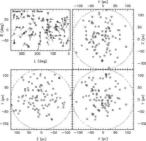
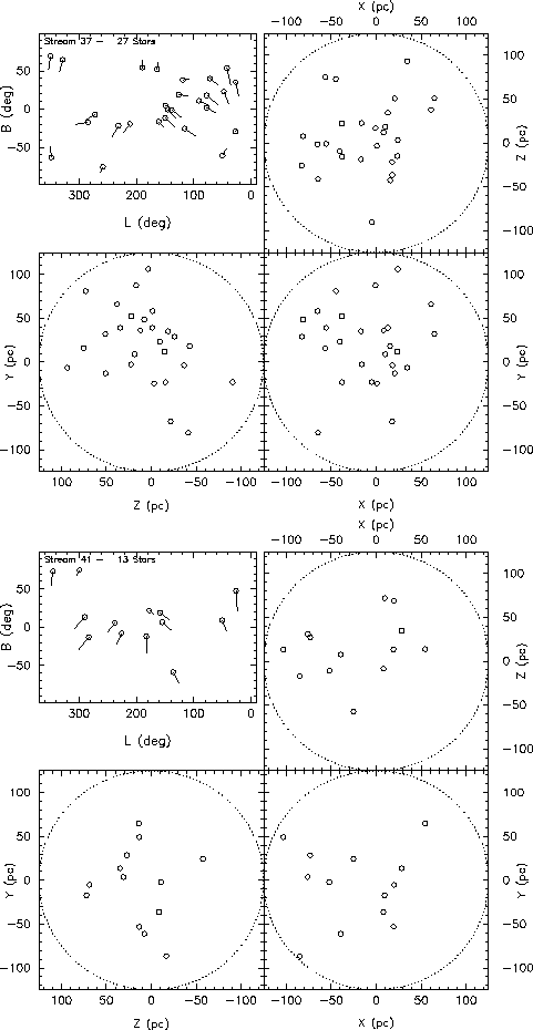
At scale 2, the supercluster splits into two distinct streams (stream 2-37 and 2-41 in Table 3) at respectively (U, V, W) = (+12.4, +0.7, -7.7) km s^-1 with ($\sigma_{U}$, $\sigma_{V}$, $\sigma_{W}$) = (4.0, 4.6, 4.7) km s^-1 and (U, V, W) = (+12.4, +4.2, -9.0) km s^-1 with ($\sigma_{U}$, $\sigma_{V}$, $\sigma_{W}$) = (3.7, 3.3, 2.9) km s^-1 producing a very clear age separation: the very young stars are separated from a part of the oldest components (6 10⁸ and 1.6 10⁹ yr). The very young component appears exclusively in stream 2-37 (middle right of Fig. 17). At the highest resolution, on scale 1 (bottom of Fig. 17), the stream 2-41 contains oldest components still interpenetrated. Space distributions (Fig. 19) show that the first stream, which contains the 10⁷ year old component is still concentrated. There are too few members in the second clump to make conclusions.

The Sirius SCl is composed by three age components of $\sim 10^{7}$, 6 10⁸ and 1.5 10⁹. The younger stream is still concentrated both kinematically and spatially while the two oldest streams are mixed in a larger volume of the phase space.

  

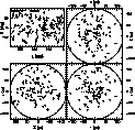Figure 18: Space distribution of Sirius SCl from the VR selected sub-sample at scale 3 (stream 3-19 in Table 2)

  

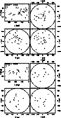Figure 19: Space distributions of the 2 sub-streams of Sirius SCl from the VR selected sub-sample at scale 2: stream 2-37 (top) and 2-41 in Table 3 (bottom)

  

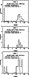Figure 20: IC 2391 SCl. Age distributions for the IC 2391 SCl (stream 2-14 in Table 3) at scale 2 (top), for sub-stream 1-20 (in Table 4) at scale 1 (middle) and for sub-stream 1-25 (in Table 4) at scale 1 (bottom)

  

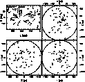Figure 21: Space distribution of IC 2391 SCl from the VR selected sub-sample at scale 2 (stream 2-14 in Table 3)

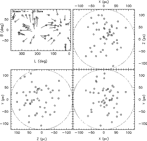
4.

IC 2391 SCl
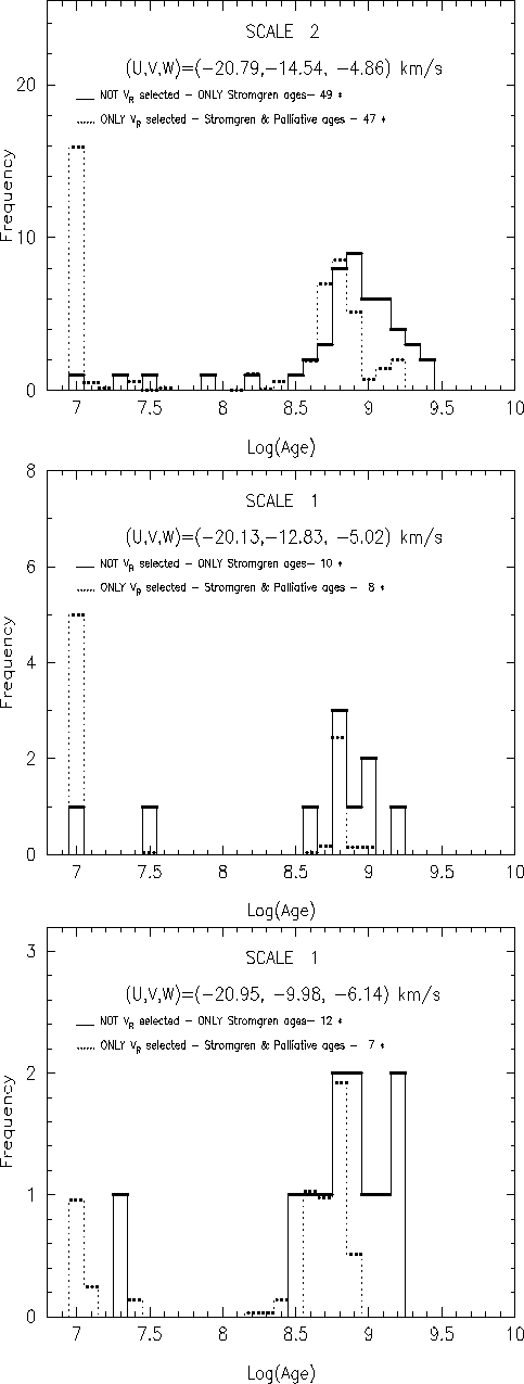
The IC 2391 SCl (see Figs. 20 for age distributions and Fig. 21 for space distributions) is not found at large scale because it may have been merged into the Centaurus association velocity group. It appears separately at scale 2 (stream 2-14 in Table 3) at (U, V, W) = (-20.8, -14.5, -4.9) km s^-1 with velocity dispersions ($\sigma_{U}$, $\sigma_{V}$, $\sigma_{W}$) = (4.3, 4.9, 5.0) km s^-1 (see Fig. 15 of Paper II). Eggen (1991) states that IC 2391 SCl contains two ages: 8 10⁷ and 2.5 10⁸ yr while Chen et al. (1997) found a mean age of $4.6 \pm$ 1.6 10⁸ yr. The Strömgren age distribution is quite different from the palliative age distribution at coarser resolution. Strömgren ages peak at 8 10⁸ but with ages up to 2 10⁹ yr. Palliative ages exhibit a peak at 6 10⁸ yr and a 10⁷ year old component (Fig. 20). This last peak is certainly real because its proportion is too high to be a statistical ghost of palliative ages from a 6 10⁸ year old component and moreover Strömgren ages show the presence of young stars. Two sub-streams are found at scale 1 (stream 1-20 and 1-25 in Table 4) at (U, V, W) = (-20.1, -12.8, -5.0) with ($\sigma_{U}$, $\sigma_{V}$, $\sigma_{W})=$ (2.9, 3.1, 1.8) km s^-1 and (U, V, W) = (-20.9, -10.0, -6.1) with ($\sigma_{U}$, $\sigma_{V}$, $\sigma_{W}$) = (4.5, 3.7, 2.9) km s^-1. The stream 1-20 contains all the youngest stars while the sub-stream 1-25 is only constituted of the 6 10⁸ year old population. Velocity dispersions of the two streams are in agreement with this view: they are smaller for the stream with the younger component. This configuration is exactly the opposite of the Pleiades' one: in this case the youngest population is more concentrated in the velocity space and is entirely detected in one stream while the oldest span over the two streams.

  

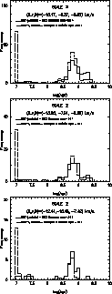Figure 22: Streams associated with Centaurus Associations. Age distributions of the overall association (stream 3-15 in Table 2) at scale 3 (top). Age distributions of Centaurus-Crux (stream 2-26 in Table 3) at scale 2 (middle). Age distributions of Centaurus-Lupus (stream 2-12 in Table 3) at scale 2 (bottom)

  

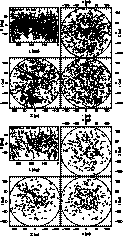Figure 23: Space distributions of the stream associated with Centaurus Associations (stream 3-15 in Table 2) for all the stars (top) and for the VR selected sub-sample (bottom) at scale 3. Stars belonging to spatial clumps in the upper figure disappear because of the lack of observed radial velocities

  

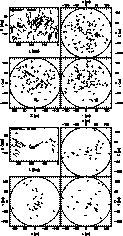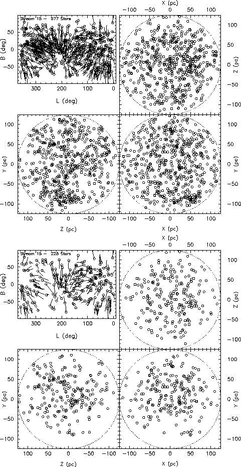
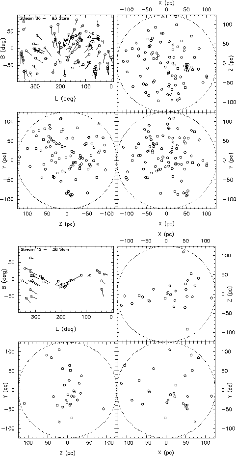
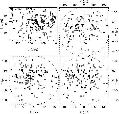
Figure 24: Space distributions of sub-streams associated with Centaurus Associations. Centaurus-Crux (stream 2-26 in Table 3) (top) and Centaurus-Lupus (stream 2-12 in Table 3) (bottom) associations from the VR selected sub-sample at scale 2. A disklike structure appears with the Centaurus-Lupus stream, on the (X, Z) projection, reflecting the Gould Belt

5.

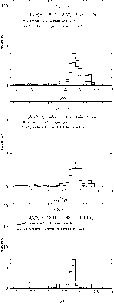
Centaurus Associations and the Gould belt
Lower Centaurus-Crux and upper Centaurus-Lupus associations (see Figs. 22 for age distributions and Figs. 23 for space distributions) which are the main components of the entire Centaurus association are detected as one velocity clump at scale 3 (stream 3-15 in Table 2) with (U, V, W) = (-15.2, -8.4, -8.8) km s^-1 with velocity dispersion ($\sigma_{U}$, $\sigma_{V}$, $\sigma_{W}$) = (8.6, 6.7, 6.1) km s^-1. Scale 3 is a too coarse resolution and the age distributions reflect the overall distribution. The whole Centaurus association is splitted into two parts at scale 2 and does not evolve at scale 1 (see Paper II, Fig. 15).

At scale 2, Centaurus-Crux (stream 2-26 in Table 3) and Centaurus-Lupus (stream 2-12 in Table 3) are identified at (U, V, W) = (-13.1, -7.9, -9.3) km s^-1 with ($\sigma_{U}$, $\sigma_{V}$, $\sigma_{W}$)= (6.2, 6.1, 5.5) km s^-1 and (U, V, W) = (-12.4, -16.5, -7.4) km s^-1 with ($\sigma_{U}$, $\sigma_{V}$, $\sigma_{W}$) = (6.1, 4.6, 3.1) km s^-1 respectively. Unfortunately, as for the Pleiades SCl, a lot of young stars have not Strömgren photometry. Strömgren age distributions peak at 6 10⁸ yr for both sub-streams but palliative age distributions show the predominance of the very young population (10⁷ yr) in each case.

There is a crucial lack of radial velocities for the spatially clustered structures Centaurus-Crux and Centaurus-Lupus: one fifth of stars have observed V_R. That is why these space clumps are visible on space distributions when taking into account all the stars of the detected streams but disappear with the sub-sample selected on observed V_R (Fig. 23). At scale 2, space distributions show that stars of the velocity substructure identified as Centaurus-Lupus association belong to a disk-like structure (see XZ projection in Fig. 24) tilted with respect to the Galactic disk. Eigenvectors of the spatial ellipsoid are calculated. The two vectors associated with the largest eigenvalues allow to define the plane of the structure, assuming it passes through the Sun. The ascending node of the intersection between this disk-like structure and the Galactic plane is $l_{\Omega}=317^\circ$ which differs slightly from usual values ($l_{\Omega}\sim 275^\circ$ to $290^\circ$, Pöppel 1997). The angle between the two planes is $i=18.8^\circ$ in agreement with previous study ($i=18^\circ - 23^\circ$).

  

Figure 25: New supercluster. Age distributions of the new moving group (stream 3-18 in Table 3) at scale 3 (top left) and the sub-stream 2-27 (in Table 3) at scale 2 (top right). Age distributions o f the sub-streams 2-35 (middle left) and 2-38 (middle right) at scale 2. Age distributions of the sub-streams 2-43 (bottom left) and 2-44 (bottom right) at scale 2

6.

A new supercluster
Close to the Sirius SCl in velocity space, located at the mean velocity (U, V, W) = (+3.6, +2.9, -6.0) km s^-1 with velocity dispersions ($\sigma_{U}$, $\sigma_{V}$, $\sigma_{W}$) = (6.8, 5.0, 6.3) km s^-1, a new massive supercluster (stream 3-18 in Table 2) is detected at scale 3 (see Figs. 25 for age distributions and Fig. 26 for spatial distribution). It contains almost twice as many members as the Sirius SCl. None of the previously known superclusters corresponds to this velocity definition. Figueras et al. (1997) indicate the presence of a velocity structure at (U, V) = (+7, +6) which they cannot confirm without doubt by their analysis and interpreted it as a possible sub-structure of Sirius SCl with a mean age of 10⁹ yr. We confirm the existence of a supercluster like structure, probably never detected before because of its low velocity with respect to the Sun. On a kinematics basis it is clearly dissociated from the Sirius SCl.

Age distributions at coarser scale are similar to the whole sample ones with ages ranging from 10⁷ to 2.5 10⁹ yr. But at least 5 sub-streams at scale 2 (see Table 3) are found to form this structure. These streams show age distributions of relatively old components. Stream 2-27 shows an unambiguous peak at 6 10⁸ yr with few 1.6 10⁹ year old stars. On the basis of velocity and age content, this stream could originate from the evaporation of the Coma OCl. Stream 2-35 has stars which are 6 10⁸, 10⁹ and 1.6 10⁹ year old on the basis of Strömgren photometry but palliative ages exhibit only one peak at 6 10⁸ yr. Stream 2-38 shows a peak at 5 10⁸ yr. Stream 2-43 has Strömgren ages between 6-8 10⁸ and few 1.6 10⁹ year old stars but the palliative ages exhibit only one peak at 8 10⁸. Stream 2-44 is clearly a 10⁹ year old group. All the few very young palliative ages in each stream are probably statistical ghost because very young Strömgren ages are never present.

Age distributions at the highest resolution (scale 1), not shown here, give exactly the same results as scale 2 but the number of stars dramatically decreases.

This structure has the same features as the previously known superclusters: a juxtaposition of several little star formation bursts at different epochs in adjacent cells of the velocity field. The correlation between velocity and age is not always obvious because these bursts (5-6 10⁸, 8 10⁸ and 10⁹ yr) are not very recent. As in the Hyades SCl case, stream velocity volumes, defined by their velocity dispersions, are substantially recovering.

Implications of these results on the understanding of the supercluster concept are discussed in Paper II.

5.3.2 Outside superclusters

 

• Small scale streams.
  While superclusters are found to split into smaller scale streams most of them corresponding to well defined age, a number of other streams are detected only at small scales. Stream 2-13 in Table 3 (Fig. 27) is a typical example of such a stream. Its age distribution shows a mono-age component of 10⁹ year old and its vertical velocity is high (W=-15.3 km s^-1). Space distribution does not fill the 125 pc radius sphere and Fig. 27 probably shows on (X, Z) and (Y, Z) projections the orbit tube in which stars are confined. Stream 2-7 in Table 3 shows also the same features with a 6 10⁸ year old component and a lower vertical velocity (W= -8.5 km s^-1).
  
    

  Figure 26: Space distributions of New SCl (stream 3-18 in Table 2) from the V R selected sub-sample at scale 3

    

  Figure 27: Stream 2-13 (in Table 3). Space (top) and age (bottom) distributions from the sub-set without V R selection at scale 2

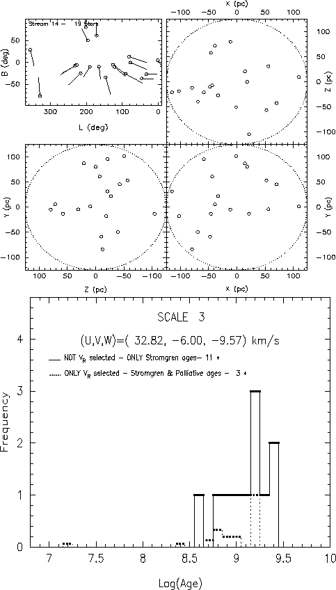
• Particulars on oldest groups.
  Another striking feature of the velocity field is the existence of a 2 10⁹ year old population still in velocity structures. These streams are only detected at the coarser resolution (scale 3) in agreement with an intrinsically large velocity dispersion. They have much less members (between 20 and 30 initial members) than the previously investigated streams and have very few observed V _R. Two main old groups (stream 3-9 and 3-14 in Table 2 and Figs. 28, 29) are clearly detected and have similar characteristics:
  
  • Age distributions peak between 1.6 and 2 10⁹ yr.
  • Their velocity dispersion obtained from the few selected stars on observed V_R are of order 6 km s^-1 (stream 3-14 seems to have a lower velocity dispersion but the result is obtained for only 3 stars).
  • U-component is positive (towards the galactic center) and often larger than 20 km s^-1.
  • Space distributions may still be clumpy.
    
    

  Figure 28: Stream 3-9 (in Table 2). Space (top) and age ( bottom) distributions from the sub-set without V R selection at scale 3

    

  Figure 29: Stream 3-14 (in Table 2). Space (top) and age ( bottom) distributions from the sub-set without VR selection at scale 3

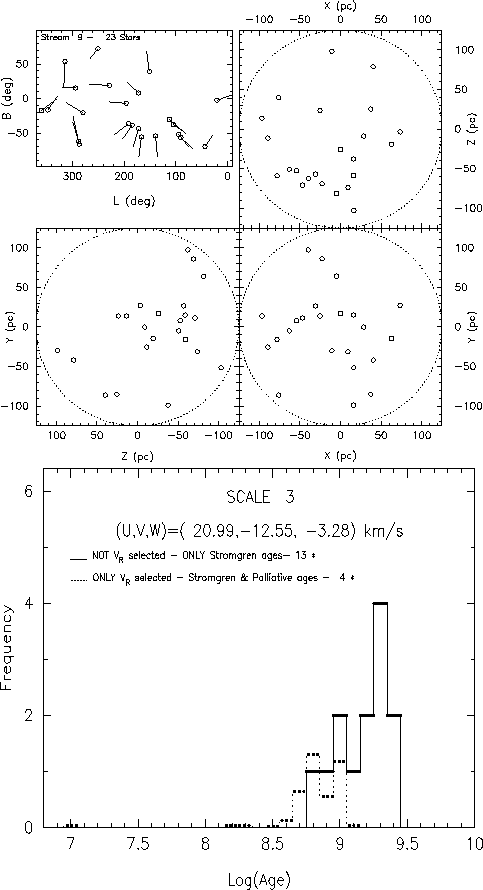
  We should notice at this point that these old star streams are both affected by two biases with respect to the whole sample characteristics. They have much less observed radial velocities (16$\%$ vs. 46$\%$) and have much more Strömgren photometry (57$\%$ vs. 37$\%$). For this reason, space distributions are displayed without radial velocity selection.

  Streams are rather fragile structures originating from cluster evaporation. The survival of these relatively old moving groups with coherent ages can be explain by two non exclusive mechanisms. On one hand, recent simulations (Zwart et al. 1998) of heavy cluster dynamical evolution (with $\sim$ 32000 particles) have shown that contrary to lighter open clusters whose typical lifetime is 1-2 10⁸ (Wielen 1971 and Lyngå 1982), heavy clusters can survive up to 4 Gyr in the Galactic gravitational field. This long lifetime can authorize to maintain old streams but such heavy open clusters are probably very rare in the disc. On the other hand, as sketched in Dehnen (1998) to explain their eccentric orbits, stars of these moving groups, provided that they were formed in the inner part of the disc, could have been trapped into resonant orbits with the non-axisymmetric force created by the gravitational potential of the Galactic bar. This latest explanation does not require any minimum lifetime to the initially bound structure from which streams originate.