2 Implementation of the wavelet analysis

 Main reasons for the choice of this algorithm developed by Holschneider et al. (1989) as well as theoretical way to compute wavelet coefficients are provided in Paper II. Here we focus on the practical computation of the wavelet coefficients (Sect. 2.1) and the thresholding procedure adopted (Sects. 2.2 and 2.3).

2.1 The "à trou'' algorithm

 

  

Figure 1: Implementation of the wavelet analysis

The adopted mother wavelet $\Psi(x)$ is defined as the difference at two different scales of a same scaling function $\Phi(x)$ (or smoothing function):  

$$\Psi(x)=\Phi(x)-\frac{1}{2}\Phi \left( \frac{x}{2} \right)\cdot$$ (1)

This particularity allows to use the "à trou'' algorithm implementation of the wavelet transform. This algorithm avoids the direct computation of the scalar product between $\Psi(x)$ and the signal F(x) to obtain wavelet coefficients. It uses an iterative schema based both on the relation existing between the mother wavelet and the scaling function (Eq. (1)) and the following relation

$$\frac{1}{2^{s+1}}\Phi \left( \frac{x}{2^{s+1}} \right) =\sum_{l=-2}^{2}h(l)\Phi \left( \frac{x}{2^{s}}-l \right)\\$$ (2)

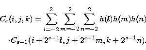
where h(l)={$\frac{1}{16},\frac{1}{4},\frac{3}{8},\frac{1}{4},\frac{1}{16}$} is a one-dimensional discrete low-pass filter. h(l) is applied in the algorithm to compute iteratively the different approximations (or smoothing) C_s of the signal at each scale s. For a 3D signal like our density or velocity distributions, h(l) is applied separately in each dimension to obtain the signal approximation at scale s and pixel (i, j, k):

$$\begin{eqnarray} C_{s}(i,j,k)=\sum_{l=-2}^{2}\sum_{m=-2}^{2}\sum_{n=-2}^{2} h(l)... ...n)\nonumber \\ \, \cdot C_{s-1}(i+2^{s-1}l,j+2^{s-1}m,k+2^{s-1}n).\end{eqnarray}$$ (3)

The distance between two bins increases by a factor 2 from scale s-1 to scale s. The result at each scale s (C_s-1(i,j,k)-C_s(i,j,k)) is the signal difference which contains the information between these two scales and is the discrete set of 128³ wavelet coefficients W_s(i,j,k) associated with the wavelet transform by $\Psi(x,y,z)$ (Fig. 1):

W_s(i,j,k)=C_s-1(i,j,k)-C_s(i,j,k).

2.2 Extracting significant coefficients

 In order to remove non-zero wavelet coefficients generated by noise fluctuations in the 3D distributions, a local thresholding is applied at each scale in the space of wavelet coefficients. Thresholds are set at each scale and each position by estimating the noise level generated at the same scale by a uniform random signal built with the same gross-characteristics as the observed one at the position considered.

• Local hard-thresholding procedure.
  The noise N_s(i,j,k) is estimated at the position of each pixel (i,j,k) from the observed distribution in a filter area corresponding to scale s. The signal estimation S_s(i,j,k), in this area, is:
  
  

  $$S_{s}(i,j,k)=\sum_{l=i-2^{s}}^{i+2^{s}} \sum_{m=j-2^{s}}^{j+2^{s}} \sum_{n=k-2^{s}}^{k+2^{s}} F(l,m,n) \\$$ (5)

  the noise estimation is:
  
  

  $$N_{s}(i,j,k)=\sqrt{\frac{S_{s}(i,j,k)}{(2^{s+1})^{3}}}\cdot$$ (6)

  At scale s, the number of pixels included in the convolution filter volume is (2^s+1)³.

  The local threshold $\lambda_{s}^{+}(i,j,k)$ is inferred from the local noise N_s(i,j,k) through calibration curves established by numerical simulations (see Sect. 2.3) which link it to the noise N_s(i,j,k). Then the hard-thresholding on wavelet coefficients follows:
  

  $$\mbox{$W_{s}(i,j,k) $}= \left\{ \begin{array} {ll} \mbox{$... ...{s}^{+}(i,j,k)$.} \\ 0 & \mbox{otherwise}\\ \end{array}\right.$$

• Segmentation procedure.
  A segmentation procedure is applied on thresholded coefficients to localize significant over-densities. This segmentation algorithm detects all maxima in a moving box of filter size volume. Neighbouring pixels are aggregated around each maximum until the intensity of wavelet coefficient stop decreasing. This is the classical method of valley lines. All aggregated coefficients around a maximum are considered to sign one structure. All structures are labelled and defined pixel by pixel. This procedure has the advantage of splitting coalescent structures.

2.3 Thresholding calibration

 

• Choice of significant probability.
  Following Lega et al. (1996), thresholds $\lambda$ are defined with respect to the probability P that the coefficient W_s(i,j,k) is larger than $\lambda_{s}^{+}$(or smaller than $\lambda_{s}^{-}$) at a given scale s in the distribution of positive coefficients (or negative coefficients).
  The probability is
  

  $$P(W_{s}(i,j,k)\geq \lambda_{s}^{+})= \frac{\int_{W_{s}=\lam... ...}} { \int_{W_{s}=0}^{+\infty} f(W_{s}){\rm d}W_{s}}=\epsilon\\$$ (7)

  where f is the frequency of positive wavelet coefficients at scale s. P was set to achieve the best compromise between false detections and losses at each scale with a set of uniform background simulations containing gaussian structures of different sizes and signal to noise ratio. This optimum was found between 5 10^-4 and 10^-4 in all experiments and in all scales under reasonable signal to noise ratio. Then $\epsilon = 10^{-4}$ was fixed for the rest of the calibration.
  
• Calibration curves.
  A calibration curve is obtained for each scale with an other set of different Poisson noise simulations. Noises N_s(i,j,k) are estimated at each pixel (i,j,k) from the observed distribution in the same way as described in Sect. 2.2. The mean $\overline{N_{s}}$ of Poisson noise distribution obtained is linked with threshold $\lambda_{s}^{+}$ (or $\lambda_{s}^{-}$) defined from P giving the calibration curve for scale s.