3 Absorption and the color-magnitude diagram

NGC 6611 is the extremely young open cluster associated with the nebula M 16. High and variable reddening and an anomalous extinction law were observed in this region (e.g. Sagar & Joshi 1979; Thé et al. 1990; Hillenbrand et al. 1993; De Winter et al. 1997). Therefore, the assumption of an average value of the color excess E_(B-V) and R_V = A_V / E_(B-V) for all cluster stars may lead to incorrect results and conclusions by a study of cluster properties.

  

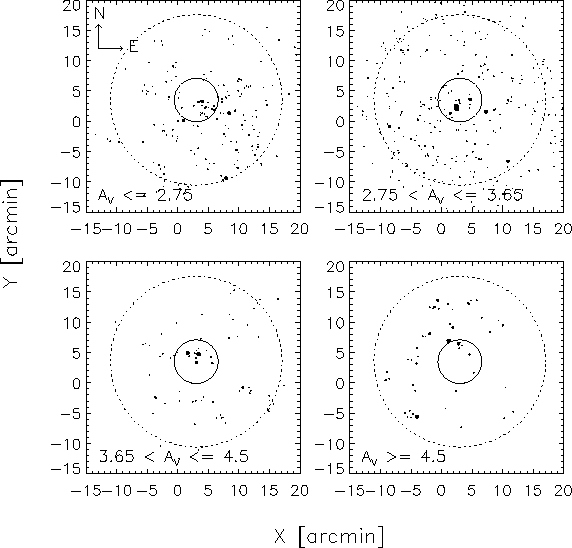Figure 8: Spatial distribution of 221 cluster members ($P({\rm pm})\gt 14\%$) belonging to the different absorption groups. Radial distances $r = 3\sigma_{X\,Y}^{\rm core}$ (solid line) and $r = 3 \sigma_{X\,Y}^{\rm corona}$ (dashed line) are also indicated. Size of filled circles is proportional to V magnitudes

3.1 Spatial distribution of absorption

In order to construct the de-reddened color-magnitude diagram for the cluster, we need to know the distributions of color excesses and R_V over the cluster area. Since data on individual values of interstellar absorption for cluster stars are rather poor, a reddening map may present a useful tool for the cluster studies. The first map of color excesses in NGC 6611 was constructed by Sagar & Joshi (1979) on the basis of 50 stars in the inner cluster region ($20 \times 20$ sq.arcmin). Our catalogue supplemented by recently published extinction data of De Winter et al. (1997) gives a basis for the construction of a new reddening map in the NGC 6611 region.

To improve the statistics of individual E_(B-V) and R_V data, we applied the Q-method technique to multicolor CCD observations of Hillenbrand et al. (1993). Stars with $Q_{UBV}<-0.43^{\rm m}$ and $(B-V) < 0.20^{\rm m}$ were taken into account and numerical parameters from Johnson (1966) and Hillenbrand et al. (1993) were used:

and

The following data sources (listed according to their priority) were included in the absorption study and reddening map construction:

• color excesses E_(B-V) from our catalogue and R_V taken from Thé et al. (1990) and De Winter et al. (1997);
• E_(B-V) and R_V calculated from Hillenbrand et al. (1993) CCD-photometry with the Q-method.

As a result, the sample for the absorption study includes 467 stars with color excesses (97 from this catalogue and 370 via the Q-method). For 174 of them, R_V determinations are available (37 from De Winter et al. 1996 and 137 from the Q-method). According to the determined membership probabilities, this sample consists of 221 probable cluster members ($P({\rm pm})\gt 14\%$) and 246 field stars ($P({\rm pm}) \le 14\%$). For the construction of the reddening map, only cluster members were considered, whereas for the R_V-map all stars with known R_V were used.

  

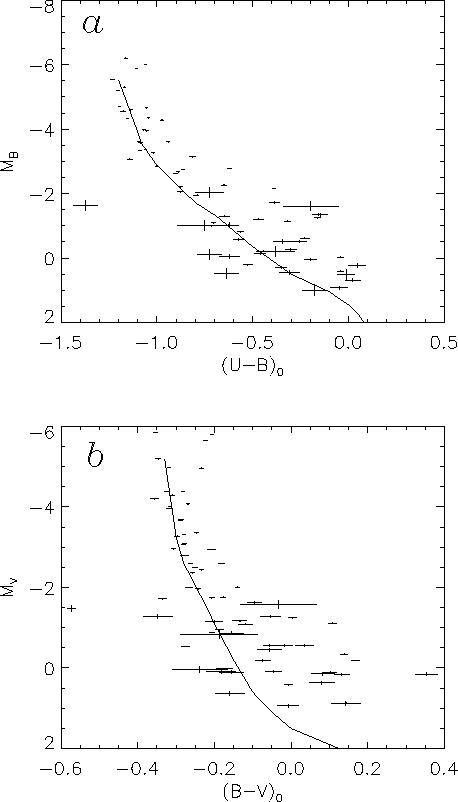Figure 9: Reddening free color-magnitude diagrams of NGC 6611 stars. Panel a) MB - (U-B)0, panel b) MV - (B-V)0. Stars with $P({\rm pm},xy) \gt 63\%$ are plotted only. Solid line is the ZAMS from Schmidt-Kaler (1982), horizontal and vertical bars indicate errors in colors and magnitudes, respectively

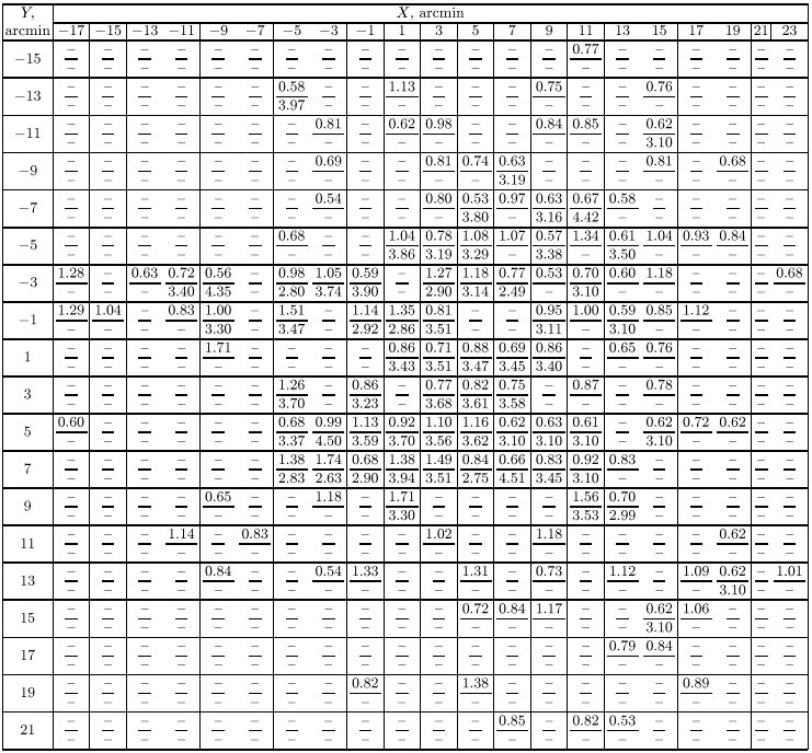
Color excesses and R_V coefficients, averaged over small cells of $2 \times 2\, {\rm sq.\, arcmin}$ are given in Table 4 (with E_(B-V) as upper line and R_V as lower line in each box). For illustration, we show in Fig. 6 the corresponding distribution of E_(B-V) over the cluster area. The map covers a sky region of $42 \times 38\,{\rm sq.\, arcmin}$ and, according to the cluster structure parameters given in Table 3, it includes both cluster core and corona.

  

Table 4: Distribution of the color excesses E_(B-V) (top) and R_V values (bottom) over the NGC 6611 region. The coordinates of the cluster centre are (X, Y) = +3.5, +3.0 which correspond to ($\alpha,\delta)_{2000.0}=18^{\rm h}18^{\rm m}40^{\rm s},-13^\circ 47.1'$

The reddening map was used to study the distribution of absorption in the NGC 6611 area. For stars with known E_(B-V) and R_V, the total absorption A_V was calculated directly from the individual values. For cluster members with R_V lacking, these values were taken, if available, from the reddening map. For remaining members an averaged value of $\overline {R_V}=3.75$ was adopted from Hillenbrand et al. (1993), whereas for field stars a value of 3.1 was assumed. The distribution of 467 stars of the sample as a function of A_V is shown in Fig. 7. A kernel density estimation method with a triangular kernel was applied to compute a smoothed distribution:

with

and i running through the sample. According to preliminary tests on the smoothing parameter h in an appropriate range of [0.1, 2.0], we chose h=1.0 as the best compromise to avoid statistical noise and to prevent an oversmoothing of the distribution.

According to Fig. 7, distributions of cluster members with proper motion probabilities $P({\rm pm}) \gt 63\%$ or $P({\rm pm})\gt 14\%$ show a similar behaviour and differ significantly from the distribution of field stars. This fact may be interpretated as an independent evidence for the correctness of the kinimatic selection procedure.

In contrast to the distribution of the cluster members, the distribution of field stars shows two distinct components. We attributed a low-absorption peak at $A_V \approx 2.5^{\rm m}$ to the foreground field, while the second peak at $A_V \approx 3.7^{\rm m}$ includes background stars highly obscured by the cluster parent cloud. Unfortunately, we cannot make more concise quantitative conclusions due to strong selection effects influencing the sample of stars with available individual E_(B-V) values.

The location of distribution features obtained for cluster candidates coincides well with the positions of the maxima of the E_(V-K)/E_(B-V) distribution in Fig. 6 of Hillenbrand et al. (1993). Assuming an average of E_(B-V)=0.79, the peaks at R_V=3.1 and R_V=3.75 correspond to $A_V=2.5^{\rm m}$ and $A_V=3.0^{\rm m}$.

Considering the local minima in the cluster member distributions over A_V, we divided 221 cluster members ($P({\rm pm})\gt 14\%$) into four absorption groups indicated in Fig. 7 by vertical lines. The spatial distribution of these stars is shown in Fig. 8. This distribution confirms a patchy behavior of absorption over the cluster. The most obscured stars are observed within a strip located to the NW of the cluster core. The less obscured group ($3.65 < A_V \le 4.5$) is randomly distributed within the core and corona whereas stars with $2.75 < A_V \le 3.65$ which could be considered as typical for this cluster unifomly fill the corona area. The stars absorbed least ($A_V \le 2.75$) mark a "transparency'' window in the SE sector of the corona. Note that stars of other groups tend to avoid the window.

3.2 Color-magnitude diagrams and distance

The magnitudes taken from our catalogue were corrected for reddening by use of individual color excesses and the redenning map. In order to determine the distance modulus of the cluster, we constructed a color-magnitude diagram (CMD) for 72 probable cluster members with a membership probability higher than 63%. Figure 9 shows both M_B -(U-B)₀ and M_V - (B-V)₀ CMDs constructed with

$$\begin{eqnarray} &&\hspace*{-3mm} M_B = M_V + (B-V)_0, {\rm~and~} \nonumber \\ && \hspace*{-3mm}(U-B)_0 = (U-B) - 0.72~E_{(B-V)}. \nonumber\end{eqnarray}$$

The ZAMS calibrations were taken from Schmidt-Kaler (1982). The distance modulus resulting from a fit of the ZAMS to the upper part of the CMDs ($M_B<-3^{\rm m}$) was derived as $(m_0-M) = 11.65^{\rm m}\pm 0.10^{\rm m}$ which is in good agreement with Hillenbrand et al. (1993) ($(m_0-M) = 11.5^{\rm m}$). The corresponding distance is $2.14 \pm 0.10$ kpc.