3 Application to the clusters of galaxies

 

3.1 A subsample of the ENACS+literature clusters

 The goal of this part is to calibrate the method with a high quality sample in order to allow a future more extensive application. We use a subsample of the regular and richest clusters of galaxies described in Adami et al. (1998) to study the variation of the galaxy aggregation with magnitude. We have used in this article COSMOS (b_j magnitude) and APM surveys (b magnitude). We keep here only the richest clusters with more than 180 galaxies brighter than b_j=20 or b=20 ($z\simeq 0.07$ and $z\leq 0.1$) in a 5 $r_{\rm c}$ area (at 5 $r_{\rm c}$ from the center, the surface density is only 1% of the central density if we assume a King profile; Therefore we have the main part of the cluster) and without apparent substructures (15 clusters). We exclude finally the clusters with an atypical King core radius (greater than 300 kpc).

We have sorted the galaxies by magnitude (b_j magnitudes). For each cluster, we select some sets of 125 consecutive galaxies out of the 180 (or more) between the $N ^{\rm th}$ and the ($N+125)^{\rm th}$ ranked galaxies. For each of those, we calculate the distance $\Delta _{m,\sigma ,s}$ and the error for this distance with the corresponding uniform sample. With N=0, 10, 20, 30, 40, 50, 60 etc., we are able to have many determinations of $\Delta _{m,\sigma ,s}$. We note however that these ranges are not independent. This allows us to compute a variation of the aggregation level with the magnitude. 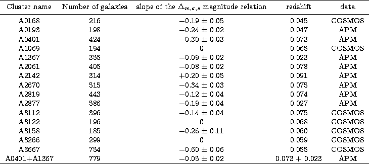We search for a negative slope, characterizing an increasing aggregation for the bright magnitudes. The selected clusters and the characteristic results are listed in Table 1.

  

Table 1: Characteristic parameters of the selected clusters: name, number of galaxies, slope of the $\Delta _{m,\sigma ,s}$/magnitude relation, redshift and type of the data (COSMOS/APM)

The clusters A1069, A3122 and A3266 have not a significant tendency at the 1 $\sigma$ level: the regression line between $\Delta _{m,\sigma ,s}$and the magnitude have a slope equal to 0. The cluster A2142 shows a positive slope (i.e. a decreasing aggregation for the bright magnitudes). The other clusters (75% of the sample) exhibit a significant decreasing tendency at the 1 $\sigma$ level.

3.2 Field contamination

  Our simulations do not take into account a possible background contribution. Such a contamination could reduce the efficiency of the discrimination. We test here two kinds of contamination: a uniform one (uniform density of background galaxies) and a clustered one (presence of secondary groups on the same line of sight).

3.2.1 Uniform contamination

 In order to test this point, we have selected the cluster A3158 in an area of 2 Mpc. According to the background level computed in Adami et al. (1998), the ratio (C hereafter) between the background galaxies and the cluster members is 3.7. In this area, the $\Delta _{m,\sigma ,s}$ distance is significantly different from 0. We are able to see the structure (Fig. 7).

We increase artificially C by uniformly adding galaxies in the selected field of view. For each set of added galaxies, we make 100 realizations in order to compute an error for $\Delta _{m,\sigma ,s}.$ We show in Fig. 7 the variation of $\Delta _{m,\sigma ,s}$ with C. We can see that $\Delta _{m,\sigma ,s}$ is significantly different from 0 (according to the error bars) for $C\leq 5$. For $5\leq C\leq 7$, $\Delta _{m,\sigma ,s}$ is different of 0 in more than 50% of the realizations. For $C\geq 7$, we are not able to distinguish the cluster structure in more than 50% of the 100 realizations.

We conclude that we are able to make the difference between the cluster and the field even if the ratio C is equal to 5, and probably 7. The influence of a uniform background level is therefore minor.

  

Figure 7: Variation of $\Delta _{m,\sigma ,s}$ for A3158 with different ratio C between the number of background and cluster galaxies

3.2.2 Clustered contamination

  The other possible contamination is that of secondary groups or clusters on the same line of sight. To test this effect, we have built a composite cluster: we have superposed the cluster A0401 (z=0.073) and the cluster A1367 (z=0.023). The contribution of A1367 will then add a signal of structure on the line of sight. We see that we destroy almost all the decrease of $\Delta _{m,\sigma ,s}$: the slope of the regression is $-0.05\pm 0.03$ (see Table 1). This kind of contamination can erase the variation of the distance $\Delta _{m,\sigma ,s}$ with magnitude.