4 The O-C diagrams of the respective systems

The analysis of the O-C diagrams for the respective ET-systems listed in Table 1 is presented in this chapter. The O-C diagrams for most of the systems are displayed to demonstrate the accuracy and reliability of the period changes, eventually the constancy of the orbital period.

Some binaries already known to display LITE (IU Aur - Mayer 1990) or seriously suspected of it (ZZ Cas - Kreiner & Tremko 1993) were rejected from the set because this effect can often preclude visibility of the "intrinsic" changes which are the target of this analysis.

4.1 V 337 Aql

The latest solution of the light curve of this system comes from Giuricin & Mardirossian (1981a) and is based on the mass ratio q=0.6 obtained from the RV measurements by Alduseva (1977). Catalano et al. (1971) reported variable light curve and possible decrease of the period length in the past. Mayer (1987) did not confirm the continuing decrease in the recent decades but admitted LITE.

The period given in SAC96 is too long. The new elements were determined and are given in Eq. (1). The O-C values for the available timings calculated according to this ephemeris are displayed in Fig. 1. Standard deviation of the photographic data is 0.011 days.

 

$$T({\rm min~I})~= 2\,441\,168.401~+ 2.733885534~E.$$ (1)

There is a tentative suggestion of a decrease of the period length within the covered interval but this trend is to a large extent dependent on the old photographic timings. While some of these old timings of the primary minima suggest longer period in the past the course of the secondary ones (probably not used in the previous analyses) may be consistent with the constant period. These photographic data (apart from one) come from a single source (Dugan & Wright 1939). The photoelectric timings are available only for a short interval. A parabolic fit of all weighted O-C values was attempted. The result is shown in Fig. 1 but it must be regarded as uncertain. It yields $\Delta$$P/P \approx-6.5\ 10^{-10}$ days$^{\rm -1}$ with S=1.9. Although this value of S is rather high, the evidence for a period decrease is based just on two old photographic timings and a single photoelectric observation, as can be inferred from Fig. 1. New observations are therefore urgently needed.

  

Figure 1: The O-C diagram for V 337 Aql. The possible parabolic trend leading to a decrease of P is marked

4.2 SX Aur

This system was classified as semi-detached by Stothers (1973) but as he noted the components are very close to each other. This conclusion was confirmed by Bell et al. (1987). The gainer almost fills in its lobe (Fig. 17a) and according to Bell et al. is evolving into contact.

The elements given in SAC96 roughly satisfy the O-C values in the second half of the data set. The examination revealed that the O-C values of the photoelectric timings spanning about 40 years can be well approximated by a straight line and allow for an improvement of the elements. The new ephemeris is given in Eq. (2) and was also used for the construction of the O-C diagram in Fig. 2. Standard deviation of the photographic and visual data is 0.003 days.

 

$$T({\rm min~I})~= 2\,445\,739.5948~+ 1.210080017~E .$$ (2)

  

Figure 2: The O-C curve for SX Aur. The photoelectric data within $E=-11\,000$ to 1900 are consistent with the constant period while the older data suggest increase of P inside the covered interval. Both parabolic fit of the whole data set and linear fit of the segment are displayed. See the text for details

It can be readily seen that the orbital period is variable and was definitely increasing during the last 82 years. Nevertheless, it is difficult to determine the exact course of this change. As was mentioned above the photoelectric data are consistent with the constant period in the last four decades. The parabolic fit of the whole data set which is displayed in Fig. 2 can plausibly match all the O-C data apart from one photoel. timing in $E= -10\,500$ which is displaced by about -7 min. The parabolic fit with S=3.19 yields the rate of the period change $\Delta$$P/P= 1.36 \ 10^{-10}$ days$^{\rm -1}$ which is in a good agreement with the value determined by Kreiner & Tremko (1978).

For the sake of completeness, a linear fit to a segment of the data within $E= -23\,050$ to $-10\,000$ was made (a long-dashed line in Fig. 2). The corresponding magnitude of the period change is $\Delta$$P/P= 2.07\ 10^{-6}$ days$^{\rm -1}$ for this case. As can be seen in Fig. 2 the data do not allow to resolve which fit is more appropriate.

4.3 TT Aur

TT Aur is a close semi-detached system (Bell et al. 1987). An extensive set of timings obtained by various methods and covering 88 years exists for this binary. The O-C values were calculated according to the elements given by Hanzl (1994). The visual inspection of the plot (Fig. 3) revealed a complicated course of the O-C values. The photoelectric timings are available for the interval of $E=-10\,000$ to 1000 (36 years). The orbital period from Hanzl (1994) satisfies the mean course of O-C values in this interval but the moment of the basic minimum needs to be shifted by -0.0054 days (see below). The new ephemeris is given in Eq. (3). Even the photoelectric data display an unusually large scatter. A detailed examination of the plot of the O-C values and consequent search for periodicity, carried out using PDM program (Stellingwerf 1978), revealed that this scatter is caused by cyclic variations on the time scale of about 12 years.  

$$T({\rm min~I})~= 2\,448\,599.2964~+ 1.332735~E .$$ (3)

  

Table 2: Orbital elements of the hypothetical third body in TT Aur determined from the photoelectric timings. A is the semi-amplitude of the O-C changes in days. T₀ is the systematic shift of the fitting. A rms error of one measurement of unit weight is 0.0008 d

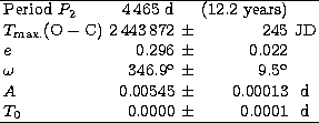Although the cyclic trend can be traced also in the means of four visual timings (triangles in Fig. 3; $\sigma=0.0047$ days) it was decided to base its analysis only on the set of thirteen photoelectric minima and one photographic timing since these changes are well defined there. The PDM program revealed two closely spaced periods: 4465 days (significance $\Theta=0.1762$) and 4286 days ($\Theta=0.1773$). The data used for this search therefore cover almost three consecutive cycles. The orbital solution found by the program SPEL showed that the O-C changes are consistent with the presence of the third body (LITE) and the period $P_{2}= 4\,465$ d was preferred since it yielded a marginally better fit. The orbital elements are given in Table 2. Both programs were written by Dr. J. Horn at the Ondrejov Observatory and details of using these programs for analysis of LITE can be found in Simon (1996). The value of eccentricity of the orbit of the possible distant companion is below the significance level given by the criterion of Lucy & Sweeney (1971) and needs to be improved by the future observations.

The systematic shift of the fitting T₀ was interactively adjusted to zero. Although the full amplitude is just about 15 min also the averaged visual data generally follow the course of the photoelectric ones, as can be seen in Fig. 3.

  

Figure 3: The O-C curve of TT Aur calculated according to the ephemeris in Eq. (3). The period changes appear to be complex. The cyclic variations are well defined by the photoelectric timings (see also Fig. 4). The means of four visual timings were used for $E\gt-10\,000$ while the individual visual observations are plotted for the older data. The solution for LITE with the parameters given in Table 2 is repeated for the whole data set. The earliest data speak in favour of a long-term increase of the period. The dot-dashed line represents the parabolic fit to the whole data set. See the text for details

The mass function of the third body is f(m$_{\rm 3}$) = 0.006405. The observed semi-axis of the eclipsing pair orbiting around the distant companion is a$_{\rm 12}$sin j = 0.99 AU where j denotes an inclination angle of the orbit of the third body. The expected semi-amplitude K(RV) of changes of the systemic velocity accompanying LITE is 2.5 km s$^{\rm -1}$ and this shift could be possibly detected in a set of high-dispersion spectra secured in the course of several years.

A set of the parametric solutions of the mass of the suspected third body in TT Aur is given in Table 3. The minimum mass of this distant companion is $1.11~M_{\odot}$ what corresponds to spectral type G3V. Its mass grows with decreasing angle j and reaches $2.50~M_{\odot}$ for $j=28.1^{\rm o}$ (B9.5V). A companion with such an early spectral type could be already revealed in the solution of the light curve as the third light. Nevertheless, such an analysis by Bell et al. (1987) did not reveal this excess light and we can therefore conclude that this companion, if present, is rather a low-mass star of medium or later spectral type.

  

Table 3: The set of parametric solutions of the mass of the third body in TT Aur. The spectral type corresponds to the appropriate mass of a main sequence star given by Harmanec (1988). The visual absolute magnitudes M_V were adapted from $M_{\rm Bol}$ in the same source and corrected for BC

The cycles with P₂ are plotted also for the earlier data in Fig. 3. The O-C values of the old data which standard deviation is 0.005 days tend to be systematically more positive within $E= -24\,500$to $-14\,500$ in comparison with the newer timings. Increase of the orbital period of the eclipsing pair can give a plausible explanation. The whole data set was fitted by a parabola and yielded $\Delta$$P/P\approx 1.2\ 10^{-10}$ days$^{\rm -1}$. This parabolic increase has significance S=1.37 (after subtraction of the cyclic variations). The O-C variations in TT Aur can be thus described as a superposition of a parabolic trend and cyclic changes.

  

Figure 4: The cyclic course of the O-C values for TT Aur folded with the period of 4465 days. The smooth curve represents the orbital solution for LITE with the parameters given in Table 2

4.4 BF Aur

This system is exceptional in this ensemble since its mass ratio q is very close to unity. Leung (1989) classified this binary as an inverse Algol (q>1) where the more massive star is more advanced in its evolution and fills in its Roche lobe while the less massive component is still inside its lobe. Kallrath & Kamper (1992) preferred a detached configuration but the more massive (but less luminous) star is still only by about 2% smaller than its lobe. Demircan et al. (1997) have recently argued that the fainter but hotter and less massive component fills its lobe; q would be smaller than unity and BF Aur would not be inverse Algol. Djurasevic et al. (1997) showed that solution with q>1 is possible, too, and Demircan et al. (1997) admitted that it is not possible to resolve between these models because they are based on the only one available set of radial velocity curves published by Mammano et al. (1974) which does not allow for exact determination of q. The solutions agree that both components are very similar to each other and also the differences in the parameters of both stars given by the respective authors are small. The parameters used in Table 1 come from Kallrath & Kamper (1992).

The available timings cover about 95 years. Since the primary and secondary minima have almost identical light curves both were used for the construction of the O-C diagram with times of the secondary minima shifted by P/2. The elements with the orbital period given in Eq. (4) (taken from SAC96) and used in Fig. 5 satisfy the second half of the covered interval while the O-C values in the first half suggest a shorter period. Standard deviations of the photographic and visual timings are 0.009 and 0.005 days, respectively.

 

$$T({\rm min~I})~= 2\,449\,002.0255~+ 1.58322190~E.$$ (4)

  

Figure 5: The O-C values for BF Aur covering about 95 years calculated according to the elements from SAC96. Both the primary and secondary minima (shifted by P/2) were used. The fits of the data are displayed. See the text for details

A change of the orbital period definitely occurred within the covered interval but since the photoelectric data are available only for about a half of the interval an exact determination of the character of this change is somewhat difficult. Both possibilities, parabolic course and constant period, are plotted for the interval of $E= -23\,000$ to $-12\,000$ in Fig. 5. Only photographic and visual timings are available there and their scatter is large therefore the resolving between parabolic course and constant period is impossible in this interval. The parabolic fit of the whole data set (S=2.25) yields $\Delta$$P/P= 1.75\ 10^{-10}$ days$^{\rm -1}$ what is in a good agreement with the value $2.07\ 10^{-10}$ days$^{\rm -1}$ determined from a much shorter segment ($\Delta$$E\approx9\,000$) by Zhang et al. (1993). This fact speaks in favour of a rather continuous period change.

4.5 AQ Cas

This binary is a very massive system ($21.3~M_{\odot}$) with long orbital period of 11.7 days. The available timings cover about 56 years. The elements given by Olson (1994) were used. They suit the data but the basic minimum should be 2426282.43 JD rather than 2426282.34 JD. The corrected value is used in Fig. 6. Standard deviation of the visual and photographic data is 0.059 days. As S=1.02 suggests the period can be considered constant within the scatter of the data.

  

Figure 6: The O-C curve for AQ Cas. The data are consistent with the constant period during the whole interval. A set of parabolas represents the expected period changes assuming the conservative case and various values of $\dot m$. See the text for details

The mass transfer rate $\dot m \approx 5\ 10^{-7}M_{\odot}~{\rm yr}^{-1}$was determined from the photometric manifestations of the mass stream by Olson & Bell (1989). In order to assess how large $\dot m$ for the conservative transfer (Huang 1963) can be hidden in the scatter of the data parabolic courses for a set of $\dot m$ were computed and are included in Fig. 6. It can be seen that the expected course of the period change for $\dot m$ determined by Olson & Bell (1989) is too small to be unambiguously present in the available data.

It is interesting to note that although the parameters and position of AQ Cas in the r-q and P-q diagrams in Fig. 17 are very similar to $\beta$ Lyr (see below) the magnitudes of the period changes are very different.

4.6 XZ Cep

The mass transfer in XZ Cep is still proceeding since the spectral lines, namely those of the Balmer series, are contaminated by CM (Glazunova & Karetnikov 1985).

The orbital period of XZ Cep is variable (Kreiner et al. 1990). These authors offered a parabolic fit of the O-C values. The timings contained in the Lichtenknecker database are the same as those analysed by Kreiner et al. (1990). The O-C values calculated according to their Eq. (3) (Fig. 7) were reexamined. The covered interval is about 57 years long and an increase of the orbital period is evident (S=2.21). Nevertheless, the character of this change is not quite clear. The O-C values within $E=2\,300$ to 4100, i.e. 25 years, are consistent with the constant period. A group of timings within E=0 to 400 has significantly more positive O-C values. Standard deviation of these mostly visual data is 0.016 days. There also exists an alternative to the parabolic trend: a possible abrupt change which took place at $E=2\,300$ or sooner. In this case a lower limit of the period change is $\Delta$$P/P\approx 0.72\ 10^{-5}$days$^{\rm -1}$. Both alternatives, parabolic fit and a lower limit of the abrupt change, are shown in Fig. 7 and as can be seen they are indistinguishable at present.

  

Figure 7: The O-C curve for XZ Cep. The data within $E=2\,300$ to 4100 are consistent with a constant period while the old data suggest increase of the period somewhere inside the covered interval. Both parabolic trend and lower limit of an abrupt change are displayed. See the text for details

4.7 V 448 Cyg

V 448 Cyg is a system with the total mass about 39 $M_{\odot}$ and the less massive secondary star fills in its lobe (Harries et al. 1997). The mass transfer is proceeding as was documented by an analysis of the emission in H$\alpha$ by Volkova et al. (1993). This emission was interpreted in terms of two components: (1) the mass outflowing through the L₂ point; (2) the mass streaming from the loser towards the gainer. The light curve is variable and the changes are prominent namely in the secondary minimum (Zakirov 1992).

The O-C values calculated according to the elements from SAC96 (Eq. (5)) are displayed in Fig. 8. Standard deviation of the photographic and visual data is 0.047 days. The total length of the covered interval is about 86 years and although there is a gap in the data the course of the O-C values is consistent with the constant period within the accuracy of the timings (S=1.11).

 

$$T({\rm min~I})~= 2\,416\,361.107~+ 6.5197162~E .$$ (5)

  

Figure 8: The O-C curve for V 448 Cyg. The whole data set is consistent with the constant period

4.8 u Her

The system is semi-detached with the primary being the main sequence star while the evolved secondary is relatively larger and overluminous for its mass (Koch et al. 1970; Eaton 1978). A difference in RVs of the triplets and singlets of HeI amounting 13 km s$^{\rm -1}$ was interpreted in terms of contamination by circumstellar material (Hilditch & Hill 1975). The gas streams were inferred from variations in the equivalent heights of the absorption lines of the primary by Kovachev & Reinhardt (1975).

A very extensive set of timings is available for this bright binary. Nevertheless, as a detailed examination showed the visual data display appreciable scatter. Since the photoelectric timings cover an interval about 73 years long it was decided to base the analysis just on these data. The period given in SAC96 was found to be too long. Its new value was determined from the moments of the primary minima in the whole covered interval and the corrected elements can be found in Eq. (6).

 

$$T({\rm min~I})~= 2\,436\,831.3040~+ 2.051026168~E .$$ (6)

  

Figure 9: The O-C values for u Her. Only the photoelectric data covering the interval 73 years long were used. The elements in Eq. (6) were used and it can be seen that the period was constant in the whole interval

The O-C values for the primary minima (Fig. 9) are fully consistent with the constant orbital period inside the whole interval (S=1.07) and confirm the finding by Kreiner & Ziolkowski (1978). The secondary minima, shifted by P/2, are displayed, too. As can be seen they are scattered more than the primary minima and may display a marginal tendency to occur later by up to 0.01 days.

4.9 VY Lac

VY Lac is a very close binary (see Fig. 17) consisting of two early-type components but the configuration of this system is based just on the light curve solution (Semeniuk & Kaluzny 1984) and no RV curves are available. The absolute masses and radii presented by these authors and listed in Table 1 are based on the statistical mass and radius of the primary component.

 

$$T({\rm min~I})~= 2\,448\,180.3474~+ 1.036243933~E .$$ (7)

  

Figure 10: The O-C curve for VY Lac. The ephemeris in Eq. (7) well satisfies the data and the period can be considered constant within the whole interval of 66 years

The orbital period given in SAC96 is too short and does not satisfy the whole data set. New elements based only on the photoelectric timings were determined and are given in Eq. (7). The total covered interval is 66 years long and it can be seen in Fig. 10 that also the older photographic and visual minima are in accordance with the elements in Eq. (7). Standard deviation of the visual and photographic timings is 0.004 days. We can conclude that the data suggest constant period in the last 66 years (S=1.00).

4.10 $\beta$ Lyr

$\beta$ Lyr is a well-known long-period (13 days) system which displays an exceptionally strong activity among the binaries which contain only non-degenerate stars. Reviews of the research of this system can be found in Sahade & Wood (1978) and Harmanec et al. (1996). Let us only note that $\beta$ Lyr displays strong emission lines in its spectrum and the large underluminosity of the gainer was interpreted in terms of a huge opaque accretion disk (Wilson 1974). The orbital period of $\beta$ Lyr is increasing at a high rate with $\Delta$$P/P= 5.997\ 10^{-7}$ days$^{\rm -1}$ and the course of the O-C changes can be well approximated by a parabola, giving the mass transfer rate of the order of $2\ 10^{-5}M_{\odot}~{\rm yr}^{-1}$ from the less massive loser onto the more massive gainer (Harmanec & Scholz 1993). They argued that the transfer in case of $\beta$ Lyr can be regarded as approximately conservative. Moreover, Harmanec and Scholz found that also an increase of the semi-amplitude of radial velocity variations of the loser as a response to its mass loss is possible.

The large optically thick disk embedding the gainer suggests large mass inflow. Although the value of the mass accretion rate onto the gainer inferred from the model of this disk by Hubený & Plavec (1991) is about five times larger than $\dot m$ determined from the O-C change by Harmanec and Scholz the agreement is not bad and confirms exceptionally large $\dot m$. Some departure from a purely conservative mode was admitted and jets of the outflowing matter were later used as an interpretation of the spectroscopic and interferometric observations by Harmanec et al. (1996).

4.11 DM Per

The elements for this system published in SAC96 were slightly corrected and the revised ephemeris given in Eq. (8) was used for calculation of the O-C values (Fig. 8). Only the photoelectric and two visual timings were used since the rest observations displayed a large scatter. The data are consistent with the constant period inside the covered interval (S=1.08).

 

$$T({\rm min~I})~= 2\,444\,855.5057~+ 2.727741844~E .$$ (8)

  

Figure 11: The O-C values for DM Per. The data are consistent with the constant period in the whole interval of the observations

4.12 IZ Per

Only relative dimensions of this semi-detached system, listed in Table 1, are available. They were determined from the solution of the light curve by Wolf & West (1993). The absolute radii and masses could not be determined since the only one RV curve of the primary, published by Yavuz (1969), leads to an unacceptably low mass of this star (only 2.4 $M_{\odot}$), much smaller than corresponds to its spectral type B3-4 determined by Wolf & West (1993) from its spectrum. Since both components are of early spectral types the RV curve affected by a line blending can be a plausible explanation for this discrepancy.

The ephemeris given in SAC96 (Eq. (9)) fits the photoelectric and visual timings within $E= -1\,300$ to 1100 (24 years) very well and the period is constant there with S=1.05 (Fig. 12). Standard deviation of the visual data is 0.010 days. Only estimates from the archival photographic plates are available for the earlier timings and their scatter is large ($\sigma=0.067$ days). Nevertheless, also these data are consistent with the constant period during the last 92 years.

 

$$T({\rm min~I})~= 2\,444\,577.5874~+ 3.687673~E .$$ (9)

  

Figure 12: The O-C curve for IZ Per. The whole data set is consistent with the constant orbital period

4.13 RY Sct

The parameters and namely the configuration of this enigmatic system are still a matter of debates. The results agree on the facts that the total mass of RY Sct is exceptionally high and that both stars are of early spectral types. The system is certainly strongly interacting and a large mass outflow even led to formation of an extended asymmetric envelope (e.g. de Martino et al. 1992).

An overcontact configuration emerged from the solution of the light curve (Milano et al. 1981). On the contrary, King & Jameson (1979) preferred a semi-detached model of the $\beta$ Lyr-type in their discussion of the spectroscopic observations. The recent analysis of the RV curves of both components by Skulskij (1992) led to a quite new value of the mass ratio q=0.301 and smaller masses of both stars than was supposed previously. His model suggests a semi-detached configuration with a huge accretion disk around the detached gainer and is similar to the model by King and Jameson. In this context it is useful to note that as was demonstrated by the models of Zola (1995) an optically thick accretion disk completely veiling the gainer in a semi-detached binary can seriously alter the results of the light curve solution and the system can even pretend a contact configuration. The contact configuration of RY Sct obtained from photometry by Milano et al. (1981) and the semi-detached model of Skulskij (1992) and King & Jameson (1979) could be reconciled in this way. In any case, new solution of the light curve of RY Sct using Zola's approach is necessary. We will therefore make use of the model by Skulskij (1992) in the following analysis.

  

Figure 13: The course of the O-C values for RY Sct calculated according to Eq. (10) (SAC96). Fit of the primary minima by the second-order polynomial is displayed, too

The previous analysis of the period changes by Milano et al. (1981) revealed that the period of RY Sct decreases. An interpretation in terms of the mass loss or transfer was offered.

The O-C values for the data available at present were calculated according to the elements from SAC96 (Eq. (10)) and are plotted in Fig. 13. Almost all timings were obtained from the photographic observations of minima (not plate estimates). Since the depth of the primary and secondary minimum is comparable timings of both are available. They are marked by different symbols in Fig. 13. The course of the O-C changes for the primary minima is somewhat better defined (standard deviation of the photographic timings 0.078 days) but it is not possible to say now if this is caused purely by observational inaccuracies or if real changes of the light curve play a role, too. The full length of the data set confirms the decrease of the period (S=1.79). The O-C values for the primary minima were fitted by the second-order polynomial, displayed in Fig. 13. The corresponding rate of the period change is $\Delta$$P/P= -3.71\ 10^{-8}$days$^{\rm -1}$. Owing to the scatter of the data determination of any more detailed course is not meaningful at present.

 

$$T({\rm min~I})~= 2\,432\,796.477~+ 11.124138~E .$$ (10)

As King & Jameson (1979) and Skulskij (1992) argued the less massive star fills in its Roche lobe and transfers mass onto its more massive companion. The course of the observed period change, that is its decrease, is in the opposite sense than would correspond to the dominant conservative mode (see also below).

4.14 RZ Sct

This binary is a long-period (15.2 days) system consisting of two evolved stars (Olson & Etzel 1994, hereafter OE94). The large radius of the evolved gainer is the reason why this binary is placed well inside the area of direct impactors in the r-q diagram despite of its long orbital period (Fig. 17, see also below). The activity connected with the mass transfer is well documented for this system: the RV curve is distorted (e.g. McNamara 1957), emission in H$\alpha$ is visible outside eclipses (McNamara 1957; Hansen & McNamara 1959), the light curve displays distorsions by the stream (Olson & Bell 1989).

The temperature of the loser is somewhat uncertain. The values given by various authors differ but agree on spectral type A. Recent solution of the light curve by OE94 yields $T_{2}=6\,418~$K. This value leads to spectral type later (about mid-F) than given in previous analyses and may shift the loser into area of stars with COL. Nevertheless, it was decided to retain RZ Sct in the ensemble, namely because of the value of $\dot m$ available for this system (see below).

The available timings cover about 77 years and the O-C values were calculated using the ephemeris given by OE94 in the first step. These authors determined the period from their photoelectric observations done in 1983 - 1990 and although their minima have not been published this period is definitely too long and yields O-C $\approx+1.6$ days for the earliest timings. After several trials it was found that the ephemeris given in Eq. (11) satisfies most of the data (Fig. 14).

  

Figure 14: The O-C curve for RZ Sct. Although the high mass transfer rate $\dot m \approx6\ 10^{-7}M_{\odot}~{\rm yr}^{-1}$ was determined by Olson & Bell (1989) the period change is very small (if any). A set of parabolas represents the expected period changes assuming conservative case and various values of $\dot m$. See the text for details

 

$$T({\rm min~I})~= 2\,436\,942.560~+ 15.19024195~E .$$ (11)

We can see that a large part of the O-C values ($E=-1\,200$ to 0) is consistent with the constant period and the scatter is formed by timings of a lower weight (standard deviation of the visual data 0.058 days). There is a possible lengthening of the period after E=0. Five visual minima after E=0, although affected by a scatter, have more positive O-C values than the earlier timings. Two photoelectric minima can be resolved around E=0; the latter has a more positive O-C value. This increase of the period length is also in accordance with the longer P found by OE94 for the interval of years 1983 - 1990. The difference between the period given by OE94 and that in Eq. (11) is $\Delta$$P/P\approx7\ 10^{-5}$ days$^{\rm -1}$.The linear fit to the minima after E=0 yields a smaller period change with respect to the period length in Eq. (11) about $\Delta$$P/P\approx 3\ 10^{-5}$ days$^{\rm -1}$. Significance S of the period change is not very low (S=1.49) but since this change is dependent to a large extent on the scattered visual data taken after E=0 it must be regarded as uncertain.

The sense of this possible period change is in accordance with the expected period variation in the dominant conservative mass transfer in a binary where the loser is less massive than the gainer. Olson & Bell (1989) determined the mass transfer rate $\dot m \approx6\ 10^{-7}M_{\odot}~{\rm yr}^{-1}$.Various manifestations of continuing mass transfer through the years cited above are available. Moreover, as can be inferred from the photometry of OE94 the shape of the light curve with the distorsion caused by the mass stream was quite stable for at least seven years. It is not therefore unreasonable to suggest that the value of $\dot m$ determined by Olson & Bell (1989) is typical for RZ Sct in the interval covered by the timings. The appropriate change of period expected for the conservative case can be then compared to the observations in the same way as for AQ Cas. The data do not contradict the increase of P which corresponds to $\dot m$ of Olson & Bell (1989).

  

Figure 15: The plot of the O-C values of Z Vul calculated using Eq. (12). The segment marked by the longer arrowed line was used for determination of this ephemeris. Both parabolic fit and a possible abrupt change of period are shown. See the text for details

4.15 V 356 Sgr

This is a massive system (16.8 $M_{\odot}$) with the orbital period 8.9 days long. The B3 primary is supposed to be critically rotating and surrounded by a geometrically thick, opaque and non-luminous disk (Wilson & Caldwell 1978). Strong UV emission lines are visible during the total primary eclipse (Plavec et al. 1984). The photometric and spectroscopic observations in the UV band obtained with IUE revealed variable eclipse light curve and non-uniform distribution of the circumstellar matter, located namely out of the orbital plane (Polidan 1989). An outflow of mass from the system was suggested.

The timings in the Lichtenknecker database contain only the data already published by Wilson & Woodward (1995). Although the number of timings is small Wilson and Woodward argued that they did not give any evidence of a significant period change and might be even consistent with a constant period, in contradiction with the evolutionary computations by Ziolkowski (1985).

4.16 Z Vul

A very extensive set of timings obtained by various methods is available for this binary. The visual timings which are the most numerous were grouped into bins of ten observations. The plot of the O-C values calculated according to the elements from SAC96 revealed clearly variable period (S=4.84). Standard deviations of the individual photographic timings and means of ten visual data are 0.004 and 0.0027 days, respectively. New ephemeris which keeps a low slope of a large part of the O-C values and thus shows the course with the best clarity was determined from the initial elements and is given in Eq. (12). The corresponding plot can be seen in Fig. 15. Although the period length definitely increased inside the covered interval it is difficult to resolve the true character of this change. Namely the photoelectric data bring some evidence for a possible episode of an abrupt change around $E=1\,100$. Both possibilities are shown in Fig. 15. The parabolic course yields $\Delta$$P/P= 2.87\ 10^{-10}$ days$^{\rm -1}$ while the magnitude of the eventual abrupt change would be $\Delta$$P/P= 2.3\ 10^{-6}$ days$^{\rm -1}$.

 

$$T({\rm min~I})~= 2\,435\,381.3844~+ 2.454926352~E .$$ (12)

The photoelectric timings in the segment marked by shorter arrowed line (after the possible episode) in Fig. 15 were used for determination of the elements which are given in Eq. (13). This ephemeris served for calculation of the O-C values which are displayed in Fig. 16.  

$$T({\rm min~I})~= 2\,447\,744.4145~+ 2.454932059~E .$$ (13)

  

Figure 16: Segment of the data from Fig. 15 showing the detail of the possible episode of abrupt period change in Z Vul. The O-C values were calculated using Eq. (13). The long-dashed line represents the course given by Eq. (12). The parabolic fit from Fig. 15 is plotted, too. See the text for details