5 Iterative flat field estimation for raster with overlap

5.1 Introduction

In order to improve the estimated flat field, we can use the fact that a sky point is seen by several pixels of the detector. We consider:

• R = number of raster positions
• a = 32² number of pixels of the detector
• u = detector overlap (u=0 for no pixel overlap, and u=1 for pixel overlap)
• N = total number of pixels in the final image.

The number of unknown variables X should be less than the number D of data. We have X = N + a (final image + flat), and the number of data is equal to $D = R \cdot a$. The final image size depends on both the overlap factor and the number of raster positions:

<I>NI> = <I>aI> + <I>aI>(<I>RI>-1)(1-<I>uI>) = <I>aI>(<I>RI> - <I>uRI> + <I>uI>) (7)

then $X = a(R - uR + u) + a \le Ra$ implies that

$$\begin{eqnarray} R \ge \frac{1+u}{u}\end{eqnarray}$$ (8)

or

$$\begin{eqnarray} u \ge \frac{1}{R-1}\cdot\end{eqnarray}$$ (9)

These relationships give only an idea of the limits, because they do not take into account effects such as transients, field of view distortion, noise, etc. As a rule of thumb, one can consider that in practice an increased number of raster positions and pixel overlap will result in a better determination of the system.

5.2 Iterative flat-field estimation

We represent the reduced data (without flat field correction) by Image(x,y,c), where x,y is the position on the detector, and c the raster position number or configuration number. From Image and from an initial flat flat₀, we can build a raster image R₀(k,l).

$$\begin{eqnarray} P\left({\rm Image \over flat_0}\right) = R_0.\end{eqnarray}$$ (10)

From the sky image R₀, we can simulate our data by applying what we call an inverse projection. We obtain the set M(x,y,c)

<I>MI>(<I>xI>,<I>yI>,<I>cI>) = <I>P^-1I>(<I>R₀I>(<I>kI>,<I>lI>)) (11)

M can be considered a model of what we should get on the detector if the true sky image is R₀. This model can be used to obtain an estimation (flat₁) of the flat. This new flat will then lead to a new raster image, R₁

$$\begin{eqnarray} P\left({\rm Image \over flat_1}\right) = R_1\end{eqnarray}$$ (12)

or in a more general way, we have the iterative flat field correction

$$\begin{eqnarray} P\left({\rm Image \over flat_{n+1}}\right) = R_{n+1}.\end{eqnarray}$$ (13)

The problem is now to find flat_n+1 knowing Image and our sky model M. The least square solution gives

$$\begin{eqnarray} {\rm flat}_{n+1}(x,y) = \frac{ \sum_c \frac{{\rm Image}(x,y,c)M... ...}(x,y,c)^2 }}{ \sum_c \frac{M(x,y,c)^2}{{\rm RMS}(x,y,c)^2 }}\cdot\end{eqnarray}$$ (14)

Furthermore, we can assume that the flat is varying with the time. Then the Eq. (13) becomes

$$\begin{eqnarray} P\left( \frac{{\rm Image}(x,y,c) }{ {\rm flat}_{n+1}(x,y,c)}\right) = R_{n+1}\end{eqnarray}$$ (15)

and if we assume a linear variation constant over the whole image, we have

$$\begin{eqnarray} P\left(\frac{{\rm Image}(x,y,c) }{ \alpha_{n+1}(c) {\rm flat}_{n+1}(x,y)}\right) = R_{n+1}\end{eqnarray}$$ (16)

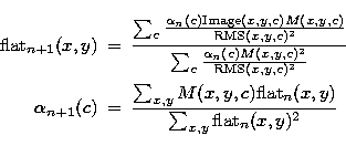
we now have one more unknown. At each iteration, we compute $\alpha_{n+1}$, and flat_n+1 by

$$\begin{eqnarray} {\rm flat}_{n+1}(x,y) & = &\frac{ \sum_c \frac{\alpha_{n}(c){\... ...} M(x,y,c){\rm flat}_{n}(x,y) }{ \sum_{x,y} {\rm flat}_{n}(x,y)^2}\end{eqnarray}$$ (17) (18)

at each iteration, the flat and $\alpha$ are normalized Simulations showed that the flat error can be divided by a factor of two (in our simulations, we derived a flat with a 5% accuracy, starting with a flat where the error was 10%). The parameter $\alpha$ is particularly useful for the first configuration when the detector is not stabilized at all.