5 Spectra of variable sources found for different observational seasons taken separately

Careful examination of Figs. 7a-c shows, however, that the representation of the dependences by a single straight lines is a strong simplification. In fact, the highest points are systematically shifted to the right from the straight lines fitting the lower points (these are shown by dashed lines). This shift mounts to 7 $\div$ 10$\sigma_V$. The F-test shows that for every graph there is the significant difference (at the confidence level 0.05) between representation the lower points by the solid and dashed lines (for solid one the dispersion is twice as large).

Because the higher points are from 1994/95 (in the flare) and the lower ones are from 1993/94 one can conclude that the properties of IR variable sources in these two time ranges were different. Therefore it is necessary to repeat the analysis for both time intervals taken separately.

Unfortunately, there are very few IR data for 1994/95. We can use the method only to K band, the value of F_K/F_V being somewhat insecure because there are only three points. Therefore we don't use this value (presented in Table 3 in brackets) in further calculations but give it only for illustration. The F-test shows that representation of the dependence in Fig. 7c by broken (dashed) line is better than by straight (solid) one at the 5-% confidence level. Thus one can be certain that in the flare the slope is flatter for all IR bands.

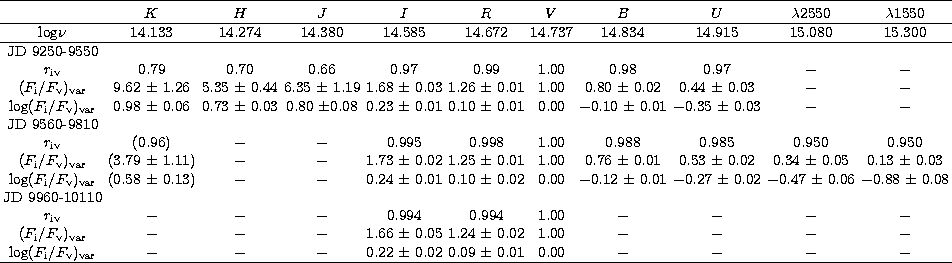
To be consistent we must divide also the optical data into different time frames. As one can see in Fig. 4 the light curve has two flares (in 1994/95 and in 1995/96). Therefore we perform the analysis for three time ranges (JD 9250-9550, JD 9560-9810 and JD 9960-10110).

  

Figure 8: The mean relative spectral energy distribution of the variable component for 1993-1996; the straight line represents only optical-UV region

The results of finding the relative spectral energy distributions of variable components for these three time ranges are given in Table 3 and shown in Fig. 9 by different symbols. Examination of Table 3 and Fig. 9 shows that all three spectra practically coincide with each other in optical region.

  

Table 3: The relative spectral energy distributions of variable sources for different time ranges

The results of fitting the data for first two time intervals in the whole available spectral range are as follows. For 1993/94 season the spectrum may be represented by straight line with the slope $\alpha = - 1.61 \pm 0.17$. Evidently the large error is due to J-band point which breaches the smoothness of the spectrum expected from physical considerations. If we exclude this point (which has the largest error!) the spectrum from K to U for 1993/94 season is well represented by straight line with the slope $\alpha = - 1.55 \pm 0.08$. Unfortunately, in this time range there are no observations of the object in extreme UV.

The spectrum in 1994/95 flare may be also represented from I to $\lambda 1550$ by straight line with the slope $\alpha = - 1.52 \pm 0.07$. Unfortunately, in the IR there is only one not too reliable point for K band. But it is evident that it lies below the straight line.

  

Figure 9: The relative spectral energy distributions of variable components for three time ranges; 1993/94 - $\bigtriangleup$(dashed line), 1994/95 - $\times$(solid line), 1995/96 - $\circ$