

Any statistical test depends on the data made of random variables. Therefore, it is necessary to know the variance of these random variables.
Throughout this paper, we only consider the cases for which random variables
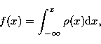
vary continuously. In this kind of cases, the cumulative distribution
function can be expressed as
 |
(10) |
 is the density function of the distribution (or the
distribution density). has the following properties:
is the density function of the distribution (or the
distribution density). has the following properties:
1  ;
;
2 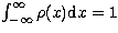 ;
;
3  .
.
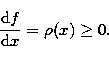
According to (10) and property 1, we have
 |
(11) |
 . The reason
is that, when
. The reason
is that, when  ,
,  is an impossible event. A sample
containing such events will not be adopted, or for such a sample, the
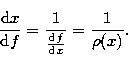
distribution will not be applied. Therefore, in the concerned intervals, f(x) must be a continuous and monotonic function of x. Thus, in these
intervals, there must exist a continuous and monotonic inverse function
is an impossible event. A sample
containing such events will not be adopted, or for such a sample, the
distribution will not be applied. Therefore, in the concerned intervals, f(x) must be a continuous and monotonic function of x. Thus, in these
intervals, there must exist a continuous and monotonic inverse function
| x=x(f) | (12) |
 |
(13) |
 |
(14) |
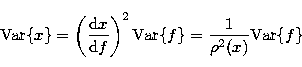
The deviation of the distribution function  of a sample from the given cumulative distribution function f(x),
  , can be considered to be caused by the deviation of
the random variable, xi,
, can be considered to be caused by the deviation of
the random variable, xi,  , from its expected value, x0i, , where
 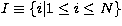 . Let
. Let
![\begin{displaymath}
x_{0i}=x[f_N(x_i)],\qquad \qquad \qquad \forall i\in I. \end{displaymath}](/articles/aas/full/1998/17/ds7271/img39.gif) |
(15) |
 |
(16) |
 |
(17) |
 |
(18) |
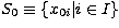 at any data point x0i, fN(x0i),
meets exactly its expected value, f(x0i), . The distribution of
S0 is exactly what would be expected from the given distribution
without any deviation. Therefore, the deviation of xi from x0i, , leads to the deviation of from f(x). Thus, from (14) we have
at any data point x0i, fN(x0i),
meets exactly its expected value, f(x0i), . The distribution of
S0 is exactly what would be expected from the given distribution
without any deviation. Therefore, the deviation of xi from x0i, , leads to the deviation of from f(x). Thus, from (14) we have
![\begin{eqnarray}
{\rm Var}\{x_i\}&=&\frac 1{\rho ^2(x_i)}{\rm Var}\{f_N(x_i)\}\n...
... &=&\frac{f(x_i)[1-f(x_i)]}{\rho
^2(x_i)N},\qquad\forall i\in I. \end{eqnarray}](/articles/aas/full/1998/17/ds7271/img44.gif) |
||
| (19) |
 distribution function deviation test for the
distribution of f(x) leads to
distribution function deviation test for the
distribution of f(x) leads to
![\begin{displaymath}
\left\vert x_i-x_{0i}\right\vert <\frac 1{\rho (x_i)}\sqrt{\frac{f(x_i)[1-f(x_i)]}N},\quad \forall i\in I, \end{displaymath}](/articles/aas/full/1998/17/ds7271/img45.gif) |
(20) |
random variable deviation
for the distribution.
One can verify that condition (20) can also be obtained by applying Eqs. (12) and (15) together with condition (9).
In the following, we present several statements concluded from Definition 1, which might be useful for statistical analysis.
Statement 1. In the cases for which random variables vary continuously, a
sample passing the distribution function deviation test
must also pass any other statistical test which depends on the deviation of
a sample from its expected value at the confidence level.
Proof. Assuming that the
random variables vary continuously, take sample  , . Let a statistical function
T of the random variables be
, . Let a statistical function
T of the random variables be
| T=T(x1,x2,......,xN). | (21) |
![\begin{eqnarray}
{\rm Var}\{T\}&=&\sum_{i=1}^N\left(\frac{\partial T}{\partial x...
... T}{\partial x_i}\right)^2\frac{f(x_i)[1-f(x_i)]}{\rho
^2(x_i)N}. \end{eqnarray}](/articles/aas/full/1998/17/ds7271/img46.gif) |
||
| (22) |
distribution function
deviation test, condition (20) is then satisfied. Therefore,

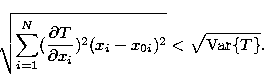 |
(23) |
Statement 2. If the random variables vary continuously, a
sample passing the distribution function deviation test
must also pass any mean-value test at the confidence level.
This statement is obvious according to Statement 1, as the mean value of any statistical function of a sample is also a statistical function of the random variables.
Statement 3. A sample passing the distribution function
deviation test also passes the Kolmogorov-Smirnov test at the confidence level.
Proof. Let sample , , pass the distribution function deviation test.
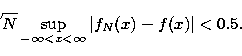
According to (9), the following relation is satisfied:
![\begin{displaymath}
\sqrt{N}\left\vert f_N(x)-f(x)\right\vert <{\sqrt{{f(x)[1-f(x)]}}.} \end{displaymath}](/articles/aas/full/1998/17/ds7271/img49.gif) |
(24) |
![\begin{displaymath}
\max \left\{ {\sqrt{{f(x)[1-f(x)]}}}\right\} =0.5, \end{displaymath}](/articles/aas/full/1998/17/ds7271/img50.gif) |
(25) |
 . Therefore,
 |
(26) |
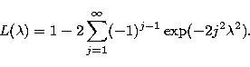
is 0.683. Let  , where
 |
(27) |
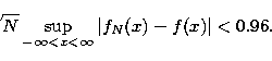
 . From (26) we find that
 |
(28) |
confidence level.
A comparison of Eqs. (26) and (28) shows that if a sample passes the distribution function deviation test, then it passes it far
better than the K-S test at the confidence level, since
 .
.
Copyright The European Southern Observatory (ESO)