4 Peak spacing and linewidth in the $l-\nu$ plane

The p-mode spectrum can conveniently be represented by a plot in the $l-\nu$ plane in which each (n,l) multiplet is represented by a point corresponding to its central frequency. In such a diagram, modes of the same n lie along clearly-defined "ridges". In order to locate the regions of the $l-\nu$ plane where modes are likely not to be well-separated from leaks, we need to know how the linewidth $\Gamma$ varies as a function of $\nu$ and l.

  

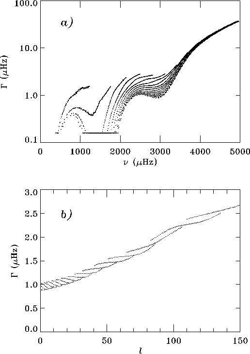
Figure 6: The approximated linewidth $\Gamma$ a) as a function of frequency $\nu$, and b) as a function of l for the frequency range $2500 \le \nu \le 3000\ \mu$Hz (where the width depends only weakly on $\nu$). The fit to $\Gamma$ is not allowed to be smaller than half a frequency resolution bin-width, i.e. 0.32 $\mu$Hz for the time series used in this plot

We illustrate in Fig. 6 the mode linewidths as observed by GONG. The linewidths have been estimated by a fitting procedure, as briefly described by Hill et al. (1996). We have then fitted to these estimated linewidths $\Gamma$, averaged over m, a sum of two cubic splines in $\nu$ and l. This provides a smooth approximation to the linewidth, which is more useful for illustrating and mapping the general trends in the $l-\nu$plane than the necessarily noisy estimates for individual modes. The GONG estimates are unfortunately available only up to l=150, because the fitting technique used is not appropriate when the ridges become blended. To fit to higher l's we need to use the leakage matrix in some way, for example as is already done for the MDI data or as described here. It is worth commenting briefly on the linewidths shown in this figure. Panel (a) shows a strong general trend for the linewidth to increase with frequency, although with a plateau between about 2200 $\mu$Hz and 3000 $\mu$Hz. This behaviour is well established observationally, as reported by, for example, Elsworth  et al. (1988), Libbrecht (1988) and Jefferies  et al. (1991), and can be approximately reproduced in theoretical calculations of damped, stochastically excited oscillations (e.g. those of Balmforth & Gough 1990 which take into account the damping associated with the coupling to convection). It is interesting that the observations indicate that the linewidth actually decreases slightly with frequency along the plateau, a feature remarked on by Balmforth & Gough and present also in their theoretical calculations. Panel (b) shows the linewidths as a function of l, over a narrow range of frequency where the frequency dependence is relatively weak. This brings out the weaker but clearly discernible trend for the linewidth to increase with degree, consistent with the observations of Jefferies  et al. (1991). The ridges of nearly connected dots in this figure correspond to modes of like n. The modes at the low-frequency end of these ridges are at higher values than one would get if one were to put a smooth fit through the high-frequency ends: this is because the figure is over a narrow range 2500 $\mu$Hz $<\;\nu\; <$ 3000 $\mu$Hz where in fact the linewidth decreases slightly with increasing frequency.

As we shall show, except at low l the closest significant leaks are from modes of the same n but with $\delta l =\pm 1$. As illustrated in Fig. 5, leaks of the same l and n, with $\delta m=\pm 2$, have no more than 25 to 30 per cent of the main peak power. In general these leaks have similar relative power on either side of the main peak where |m/l| is small, and are weak where |m/l| is large. Ideally these "m-leaks'' ought to be taken into account in fitting, but they are usually neglected. To see how the leaks affect the analysis of power spectra, we need to examine individual spectra or "$m-\nu$'' diagrams that map the power in spectra of a given l as a function of m and frequency. Plotting the data for high l spectra in this way reveals that each "ridge'' of power at a given l and n is flanked by weaker ridges of power leaked from spectra of adjacent l, as illustrated in Fig. 7. Further examples of spectra and $m-\nu$ diagrams can be seen in Hill et al. (1996). The solar rotation shifts peaks of different m away from the central frequency. Roughly speaking, the slope of the (l,n) ridges in $m-\nu$ space reflects the mean rotation rate; the slight S-shaped curvature of the ridges arises from the differential rotation, which provides important information about the variation of the rotation rate with latitude and depth. In order to derive a useful "m-averaged spectrum'' we first need to remove the m-dependence of the mode frequencies.

  

Figure 7: A greyscale plot showing a portion of the GONG month 4 power spectrum for l=150 in the $m-\nu$ plane

We can write the difference in frequency between modes that have the same value of n but degrees l differing by 1 as a derivative $(\partial\nu/\partial l)_n$, although $\nu(n,l)$ is not strictly speaking a continuous function.

  

Figure 8: An $l-\nu$ diagram showing contours of $(\partial\nu/\partial l)/\Gamma$. Each dot represents the mean position of an (n,l) multiplet, each ridge of dots corresponding to a single value of n. Fitting of modes becomes substantially more difficult outside the $(\partial\nu/\partial l)/\Gamma = 2$ contour, which is shown as bold

  

Figure 9: An $l-\nu$ diagram illustrating the regions where n-leaks are a potential problem. The different symbols show modes affected by leaks within $2\Gamma$ for various $\delta l$: $\delta l =\pm 1$ for crosses, $\delta l=\pm 2$ for triangles, $\delta l=\pm 3$ for stars, $\delta l=\pm 4$ for diamonds and $\delta l=\pm5$ for squares. The curve shows the $(\partial\nu/\partial l)=2\Gamma$ contour

Contours of $\Gamma^{-1}\partial\nu/\partial l$ are shown in Fig. 8. We anticipate particular difficulty in fitting peaks independently when this ratio is less than 2. This occurs at high frequency (around $3500-4000~ \mu$Hz), because the linewidths become large, and also at high degree ($l{\leavevmode\kern0.3em\raise.3ex\hbox{$\gt$} \kern-0.8em\lower.7ex \hbox{$\sim$}\kern0.3em}150$) where $\partial \nu / \partial l$ becomes small. The latter tendency can be seen from the approximate formula for medium and high l,

$$\omega^2 = gk(n+\alpha)$$ (7)

(e.g. Deubner & Gough 1984), where k = l/R, g is the gravitational acceleration, R is the solar radius and $\alpha$ is a constant of order unity. From this formula,

$$\left({\partial\nu\over\partial l}\right)_n\ \simeq\ {\nu\ov... ...\nu\over\partial n}\right)_l\ \simeq\ {\nu\over 2(n+\alpha)}\;,$$ (8)

assuming that g is constant. This indicates that at fixed $\nu$, the spacing $\partial \nu / \partial l$ decreases with l. (In fact the effective gravitational acceleration increases with decreasing turning point radius for modes of medium and high degree - because going down through the convection zone the interior mass decreases more slowly than r^-2 increases - so the above formulae overestimate $\partial \nu / \partial l$ and underestimate $\partial\nu / \partial n$, though they are good for order-of-magnitude and qualitative behaviour.) The above approximation implies $(\partial\nu/\partial n)/(\partial\nu/\partial l) \simeq l/(n+\alpha) .$Since $\alpha$ is of order unity, it follows that at moderate and high degree (where $l\gg n$) the frequency spacing between neighbouring n's is much greater than between neighbouring l's. The ratio decreases however as l decreases, so that at low degree it is necessary to be concerned also with nearby leaks from modes of different order n. At the lowest degrees, a more appropriate approximation for the frequencies is the Tassoul formula $\nu\ \simeq\ (n+l/2+\epsilon)\nu_0$where $\nu_0 \approx 140\,\mu$Hz and $\epsilon$ are constants, whence it can be seen that

$$(\partial\nu/\partial n)/(\partial\nu/\partial l) \simeq 2\;.$$ (9)

In the case where $(\partial\nu/\partial n)/(\partial\nu/\partial l) \le \Delta l$($\Delta l = 2,3,\cdots$), one needs to be aware of the possibility of "n-leaks'' - neighbouring modes with different radial order n - for $\vert\delta l\vert \le \Delta l$. Where $(\partial\nu/\partial n)/(\partial\nu/\partial l)$ is very close to $\Delta l$, leaks with $\delta l = \pm \Delta l$ will be particularly problematic. In Fig. 9 we show the modes whose nearest neighbour is within two linewidths: different symbols are used to show the modes affected by particular leaks. In addition to all the modes with $\delta\nu/\delta l < 2\Gamma$ (crosses), for which the nearest significant leak generally has l differing from the target degree by one, this figure indicates that there are difficulties at moderately low degree due to leakage from modes with different n (and hence - to have similar frequency to the target mode - with degrees l differing from the target degree by more than one). Note that the leakage decreases fairly quickly with $\vert\delta l\vert$, and is typically less than one per cent of the mode power at $\vert\delta l\vert = 5$.Thus leaks from modes with substantially different values of l are not a principal concern.