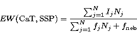
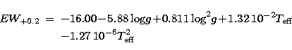
We calculate the integrated equivalent widths for the CaT lines by combining the individual stars in each evolutionary stage, according to the theoretical isochrone. To this purpose let Ij be the intensity in absorption of the two lines of CaT for each star, j, found in the HR diagram of an SSP:
| Ij = fj EWj | (1) |
where fj is the corresponding flux at the wavelength of 8600 Å for the star in the HR diagram. This quantity is obtained by a linear interpolation between the two central values of the continuum band-passes as defined by DTT89. The fluxes come from a suitable stellar atmosphere model and have been scaled to the luminosity of the corresponding theoretical star in the HR diagram. EWj is the equivalent width of CaT for a star in the evolutionary stage j, that we assume is known. If Nj describes the number of stars in the evolutionary stage j and N is the total number of points in the HR Diagram, the synthesized equivalent width of CaT for an SSP at a given epoch is:
 |
(2) |
where ![]() is the nebular continuum at 8600 Å corresponding to the SSP.
In the following both theoretical (grid I) and empirical (grid II) fitting
functions have been used to obtain the index as a function of the stellar
physical parameters:
is the nebular continuum at 8600 Å corresponding to the SSP.
In the following both theoretical (grid I) and empirical (grid II) fitting
functions have been used to obtain the index as a function of the stellar
physical parameters: ![]() , logg and abundance. The theoretical stellar
grid of EW(CaT) is from JCJ92, while the empirical library is from DTT89
plus the M type stars from Z91's atlas. We consider EW(CaT) to be
zero for stars hotter than 6700 K which is the observational limit of
DTT89's atlas.
, logg and abundance. The theoretical stellar
grid of EW(CaT) is from JCJ92, while the empirical library is from DTT89
plus the M type stars from Z91's atlas. We consider EW(CaT) to be
zero for stars hotter than 6700 K which is the observational limit of
DTT89's atlas.
JCJ92 computed a complete grid of NLTE models for the equivalent widths of
CaT lines from stars with ![]() ranging between 4000 and 6600 K,
logg between 0.00 and 4.00, and calcium abundances between 0.1 and 1.6
solar. From their models, the following fitting functions can be used to
calculate the theoretical value of EW(CaT) as a function of
ranging between 4000 and 6600 K,
logg between 0.00 and 4.00, and calcium abundances between 0.1 and 1.6
solar. From their models, the following fitting functions can be used to
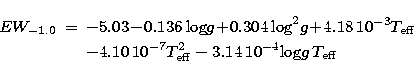
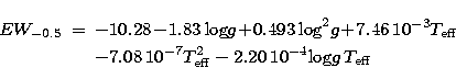
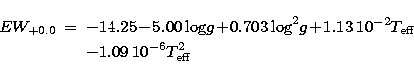
calculate the theoretical value of EW(CaT) as a function of ![]() , logg,
and calcium abundance, [Ca/H] = -1.0, -0.5, 0.0 and +0.2 (Eqs. (3),
(4), (5) and (6) respectively).
, logg,
and calcium abundance, [Ca/H] = -1.0, -0.5, 0.0 and +0.2 (Eqs. (3),
(4), (5) and (6) respectively).
 |
||
| (3) |
 |
||
| (4) |
 |
||
| (5) |
 |
||
| (6) |
![\begin{figure}
\begin{center}
\includegraphics [width=8.8cm,height=10cm]{vargas3.eps}
\end{center}\end{figure}](/articles/aas/full/1998/12/ds1379/img32.gif) |
Figure 3:
Comparison between data and models of EW(CaT) in stars. Panel a)
shows the EW(CaT) as a function of the gravity. Open circles represent data
from DTT89. Solid lines correspond to JCJ92's fitting functions for the
values of the effective temperature labelled in the figure. The dotted line
is our fit to DTT89's data, which has been used in the models (grid II).
Panel b) shows the EW(CaT) as a function of the effective temperature for
the coolest stars. For stars cooler than 4000 K, we have extrapolated the
expressions given by JCJ92 for stars with |
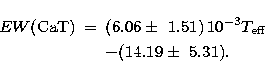
In the second grid of models we made use of the observational data
collected by DTT89 complemented by data of M-late type stars from Z91.
DTT89 provide the following relation between EW(CaT), gravity and stellar
abundance as measured by [Fe/H]:
| |
(7) |
For models with Z=0.02 and Z=0.05, we have fitted the observational
data of the EW(CaT) as a function of the gravity, following Eqs. (8)
and (9).
| (8) |
| (9) |
As already anticipated, for M-late stars we adopted the data by Z91, since these stars were not included in DTT89's library. The data given by Z91 have been converted to DTT89's system through the following relation, which has been obtained by fitting a linear regression to 20 common stars in Z91 and DTT89:
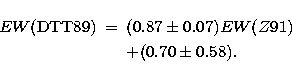 |
||
| (10) |
 |
||
| (11) |
With the above fitting functions we computed the synthetic equivalent
widths for the two main lines of CaT at ![]() Å at the four selected metallicities: 0.2
Å at the four selected metallicities: 0.2 ![]() , 0.4
, 0.4 ![]() ,
, ![]() and 2.5
and 2.5
![]() . The results are shown in Fig. 4 and the values are given in
Tables 3, 4 (grid I), 5 and 6 (grid II). For each table, Col. (1) lists
the logarithm of the age of the SSP (in yr), Col. (2) the continuum
luminosity (in units of
. The results are shown in Fig. 4 and the values are given in
Tables 3, 4 (grid I), 5 and 6 (grid II). For each table, Col. (1) lists
the logarithm of the age of the SSP (in yr), Col. (2) the continuum
luminosity (in units of ![]() ) from the SSP (nebular emission not
included), taking an average value in the DTT89's spectral band-passes;
Col. (3) the luminosity, in units of
) from the SSP (nebular emission not
included), taking an average value in the DTT89's spectral band-passes;
Col. (3) the luminosity, in units of ![]() , absorbed in the Ca II lines
at 8542 and 8662 Å by the stars of the SSP, and Col. (4) the
equivalent width of CaT, in Å, computed as the ratio between Col. (3)
and the total continuum luminosity (in which both the stellar and the
nebular contribution are taken into account). Columns (5), (6) and (7) are
the same of (2), (3) and (4) respectively, but for a different metallicity.
, absorbed in the Ca II lines
at 8542 and 8662 Å by the stars of the SSP, and Col. (4) the
equivalent width of CaT, in Å, computed as the ratio between Col. (3)
and the total continuum luminosity (in which both the stellar and the
nebular contribution are taken into account). Columns (5), (6) and (7) are
the same of (2), (3) and (4) respectively, but for a different metallicity.
| Figure 4:
Computed models for the CaT index as a function of the age of the SSP
in a logarithmic scale. Panels a), b), c),
and d) display the results for
metallicities 2.5 |
Copyright The European Southern Observatory (ESO)