10. Integrated starlight

10.1. Model predictions based on star counts

The combined light from unresolved stars contributes to the sky brightness from the ultraviolet through the mid-infrared, with the contribution being dominated by hot stars and white dwarfs at the shortest wavelengths, main sequence stars at visual wavelengths, and red giants in the infrared (Mathis et al. 1983). The integrated starlight contribution to the sky brightness depends on the ability of an experiment to resolve out the brightest stars, which in turn depends on the Galactic latitude. If we suppose that stars brighter than flux F₀ are resolved and excluded from the diffuse sky brightness, then the integrated starlight contribution is the integral over the line of sight of the brightness contributions from stars fainter than F₀,
 
where is the number of stars in the flux range F to , for a line of sight towards galactic coordinates l,b. In principle, we must also integrate the counts over the beam and divide by the beam size, but in practice, the variation in the number of sources over a beam is often small except for large beams at low galactic latitude. (In those cases, Eq. (28 (click here)) is replaced by
 
where is the beam solid angle.) The cumulative number of sources increases less steeply than 1/F for the fainter stars, so that the integral converges; in the near-infrared at 2.2 m, the peak contribution to the sky brightness occurs for stars in the range 0 < K < 6. For reference, K=0 corresponds to Jy (Campins et al. 1985), and there is of order 1 star per square degree brighter than K=6, and (extrapolating) there is one star per square arcminute brighter than K=15. Thus, for comparison, the DIRBE survey ( beam, K=4 detection limit) resolves about 50% of the starlight in the K band, while the DENIS survey (limiting magnitude K=14) should resolve some 97%. Similarly, in the far-ultraviolet, the FAUST survey resolves some 96% of starlight (Cohen et al.  1994). And at visible wavelengths, star counts near the North Galactic Pole (Bahcall & Soneira 1984) also show that the visible surface brightness for low-resolution observations is strongly dominated by the brightest stars (). It is for deep surveys with low angular resolution that we address the remainder of this discussion of integrated starlight.

To estimate the contribution of integrated starlight to a deep observation, one must sum the contribution from each type of star along the line of sight. One may recast the integral in Eq. (28 (click here)) more intuitively by integrating over the line of sight for each class of object (which has a fixed luminosity):
 
where n_i is the number density and L_i the luminosity of sources of type i. The integral extends outward from a given inner cutoff s_i that depends on the source type through . Bahcall & Soneira (1980, 1984) constructed such a model, with the Galaxy consisting of an exponential disk and a power-law, spheroidal bulge. The shape parameters (vertical scale height and radial scale length of the disk, and bulge-to-disk density ratio) of the Galactic star distribution were optimised to match the star counts. A more detailed model (SKY), both in terms of Galactic shape and the list of sources, has been constructed by M. Cohen and collaborators (Wainscoat et al.  1992; Cohen 1993, 1994; Cohen et al.  1994; Cohen 1995).

Examples of the surface brightness predicted by the SKY model for two lines of sight and four wavebands, from the ultraviolet to the mid-infrared, are shown in Fig. 61 (click here). Of these, the basis for the ultraviolet part is discussed in more detail in Sect. 10.2.2 below. Each curve in Fig. 61 (click here) gives the fractional contribution to the surface brightness due to stars brighter than a given magnitude. The total surface brightness for each wavelength and line of sight is given in Table 24 (click here). The sky brightness due to unresolved starlight can be estimated for any experiment given the magnitude limit to which it can resolve stars. First, determine the fraction, f, of brightness due to stars brighter than the limit using Fig. 61 (click here). Then, using the total brightness of starlight, from Table 24 (click here), the surface brightness due to unresolved stars is . - For specific results of the SKY model contact Martin Cohen directly.

The old compilations of integrated starlight in the visual by Roach & Megill (1961) and Sharov & Lipaeva (1973) do not have have high ( 1) spatial resolution and are not calibrated to better than 15%. However, they still give useful information, are conveniently available in tabulated form, and have been used, e.g. in work to be discussed below in Sects. 11.2 (click here) and 12.2.1 (click here).

   

0.1565 62 24

0.55 577 250

2.2 205 105

12 6.1 3.0

Table 24: Surface brightness due to integrated starlight (given as , respectively )

  
Figure 61: Fraction of integrated starlight due to stars brighter than a given magnitude, for two lines of sight: the NGP (dashed curves) and a region at galactic latitude (solid curves). Each panel is for a different wavelength: a) 1565 Å, b) 5500 Å, c) 2.2 m, and d) 12 m. In panel c), the vertical lines indicate the magnitude limits adopted in analysis of DIRBE (Arendt et al.  1997), IRTS (Matsumoto et al.  1997), and DENIS (Epchtein 1994, 1997) observations are shown

10.2. Ultraviolet

10.2.1. Near ultraviolet (180 nm - 300 nm)

The UV astronomy experiment S2/68 (Boksenberg et al. 1973) provided catalogs of stellar UV brightness over the sky in one photometric channel at 274 nm ( = 30 nm) and three spectroscopic channels around 156.5 nm ( = 33 nm), 196.5 nm ( = 33 nm), and 236.5 nm ( = 33 nm). Gondhalekar (1990) integrated over the spectroscopic channels to provide photometric information at all of the four UV wavelengths. The photometric accuracy is 10%. Only the 47039 stars with UV flux larger than ergcm^-1s^-1sr^-1Å^-1 ( 8 mag) in at least one of the four passbands were kept for calculating the integrated starlight brightness over the sky. The resulting brightnesses are given in Tables 25 (click here) to 28 (click here).

Brosch (1991) also attempted to produce a galaxy model for the UV. He adapted the Bahcall & Soneira (1980) galaxy model by suitable colour relations to the sky, and added Gould's belt and white dwarfs. He compared in his Fig. 3 the model with the limited results available from a wide field UV imager flown on Apollo 16 (Page et al. 1982) and found reasonable agreement between his model and these data, but otherwise does not give an explicit description of the model.

   
Table 25: The intensity of stellar UV radiation at 156.5 nm in bins of in units of 10^-10 Wm^-2sr^-1m^-1, respectively 10^-11 ergcm^-1s^-1sr^-1Å^-1. The limits of the bins are given in degrees of galactic logitude and galactic latitude with the table. Only stars brighter than a certain flux limit (see text) were included. From Gondhalekar (1990)

   
Table 26: The intensity of stellar UV radiation at 196.5 nm in bins of in units of 10^-10 Wm^-2sr^-1m^-1, respectively 10^-11 ergcm^-1s^-1sr^-1Å^-1. The limits of the bins are given in degrees of galactic logitude and galactic latitude with the table. Only stars brighter than a certain flux limit (see text) were included. From Gondhalekar (1990)

   
Table 27: The intensity of stellar UV radiation at 236.5 nm in bins of in units of 10^-10 Wm^-2sr^-1m^-1, respectively 10^-11 ergcm^-1s^-1sr^-1Å^-1. The limits of the bins are given in degrees of galactic logitude and galactic latitude with the table. Only stars brighter than a certain flux limit (see text) were included. From Gondhalekar (1990)

   
Table 28: The intensity of stellar UV radiation at 274 nm in bins of in units of 10^-10 Wm^-2sr^-1m^-1, respectively 10^-11 ergcm^-1s^-1sr^-1Å^-1. The limits of the bins are given in degrees of galactic logitude and galactic latitude with the table. Only stars brighter than a certain flux limit (see text) were included. From Gondhalekar (1990)

10.2.2. FUV (91.2 nm - 180 nm)

Table 25 (click here) discussed in the last subsection actually belongs to the FUV range.

As far as modelling is concerned, the stellar contributions to the FUV sky brightness have been well characterized. The optical and infrared SKY model of Cohen (1994) has been expanded into the FUV by fitting it to observations on the FUV sky obtained with the FAUST FUV telescope (Bowyer et al. 1993). The FAUST camera had obtained observational data on 5000 sources in 21 separate fields in the bandpass. These data covered FUV magnitudes from 5 to 12. The model resulting from the comparison to these data (Cohen et al. 1994) provides an excellent fit to the available FUV observations. The extrapolated flux for magnitudes greater than 12 is less than 4% of the total point source flux and is less than 1% of the FUV diffuse sky brightness.

As is the case for other wavelength bands, the integrated starlight in the FUV (and also the near ultraviolet) is concentrated toward the plane of the Galaxy. In Fig. 62 (click here) we display two examples of how the model accounts for the stellar contribution in the ultraviolet (kindly provided by Martin Cohen). The figure shows differential star counts as a function of a FUV magnitude centered at 166 nm, both for a position in the galactic plane at and for the galactic pole. In both parts of the figure, the solid line is the total number of stars per square degree per magnitude interval, the disk component is shown by the faint dotted line, and the dash-dot line is the halo contribution. For the galactic plane (left diagram), the halo component is of lesser importance, but the spiral arms plus local spur contribution have to be taken into account (long-dashed curve). Table 29 (click here) gives the total stellar surface brightness in the band as a function of galactic latitude. The brightness varies with galactic longitude; in this case we show the values for l = 90.

In an attempt to unify the above information on ultraviolet integrated starlight, at present we suggest to rely on Tables 25 (click here) to 28 (click here) for the absolute and total brightness level, and to use the models demonstrated above for purposes like extrapolation to the contribution of faint stars or breakdown of the total brightness into the contribution of different components or brightness intervals.

  
Figure 62: Differential star counts as a function of FUV magnitude for a position in the galactic plane at (left) and for the galactic pole (right). Solid line: total contribution, faint dotted line: disk component, dash-dot line: halo contribution, long-dashed line: spiral arms plus local spur (shown only for the field in the galactic plane)

   

Galactic I

latitude photons/cm²ssrÅ

26.6 0.01 102 10^-10

40.6 0.02 156 10^-10 125.8

49.7 0.03 191 10^-10 153.8

58.2 0.03 224 10^-10 180.4

70.9 0.05 273 10^-10 219.5

89.8 0.19 345 10^-10 278.0

122.1 0.3 469 10^-10 378.2

185.0 0.6 709 10^-10 571.1

483.0 12.9 1860 10^-10 1496

429.7 7.8 1650 10^-10 1330

Table 29: Total integrated surface brightness in the range due to point sources, as given by the SKY model^a at a galactic longitude of 90 as predicted by the SKY model

^aSince this model was primarily constructed for the infrared, it cannot be expected to be accurate in the ultraviolet at low galactic latitudes (), where the effects of clumpiness of the interstellar medium get dominating (Caplan & Grec 1979).

10.3. Ground-based UBVR photometries

Besides airglow and zodiacal light, the Milky Way is the third major contributor to the diffuse night sky brightness in the visual spectral domain. Its light is fixed with respect to an inertial system of reference and also is constant over large time scales. For absolute brightness determinations, space experiments, free of disturbance by the earth's atmosphere, are best suited, for studies of structures, ground-based surveys are preferable because of their greater flexibility. In any case one has to be aware of the presence of diffuse galactic light which on the average contributes between 20% and and 30% of the Milky Way brightness.

Efforts to describe the distribution of the Milky Way's brightness are numerous and can be traced back far into the past (Ptolemy's Almagest). Difficulties to get rid of atmospheric disturbances still are present in the classical paper by Elsässer and Haug in 1960, which otherwise, for the first time, presented photoelectric measurements of our Galaxy with a reasonable resolution in well defined passbands (see Tables 30 (click here) and 31 (click here)).

   

longitudes latitudes

P, V Elsässer & Haug (1960) Smith et al. (1970)

U Pfleiderer & Mayer (1971)

B Classen (1976)

Northern Milky Way Zavarzin (1978) Weinberg (1981)⁺ Weinberg (1981)⁺ Winkler et al. (1981)

B-R = 440 nm - 640 nm Toller (1990)⁺

B, V Wicenec (1995)⁺, Wicenec & van Leeuwen (1995)⁺

Table 30: Large scale surface photometries of the Milky Way in the visual/near visual spectral domain (in addition to those displayed as Figs. 63 (click here)- 67 (click here))

^*as far as visible from about 30 southern geographical latitude,
⁺space experiments, included here for comparison, see a detailed presentation of Pioneer 10 results in Sect. 10.4.
Note: The earlier photometries by Elsässer and Haug and by Smith et al. are included here only for comparison. It is recommended to refer to the space-based photometries, to the Bochum photometries shown in Figs. 63 (click here)-67 (click here) and to the later photometries of this table.

   

longitudes latitudes

B Mattila (1973)

U Pröll (1980)

U, B, V Scorpius Hanner et al. (1978)^a

U, B, V selected scans Leinert & Richter (1981)^a

U, B, V, R Seidensticker et al. (1982)

Table 31: Surface photometries covering smaller areas of the Milky Way

^a space experiment, included here for comparison, since well-calibrated.

is the wavelength which bisects the recorded energy for this filter, the equivalent width and the total width of the passband.
Please note: 1 mean errors given only if data permit (muliplicative term) and/or mean differs by more than 1 from zero (additive term).
The Bochum UBVR photometries are stored at the Strasbourg Centre de Données Stellaires (CDS) under http://cdsweb.u-strasbg.fr/htbin/myqcat3?VII/199/

The four photometries of the Southern Milky Way presented here in colour as Figs. 63 (click here)-67 (click here) profit from the now more effective correction for the atmospheric effects. They cover the whole range in longitudes and galactic latitudes from to +40. They have a high angular resolution ( square degrees). Moreover, all wavelength bands are processed in the same way, and so the colours U-B, B-V, V-R should be quite coherent. The figures presented here only give an overview, although the linear scale of the colour bar will allow coarse interpolation. The data are accessible in digital form at the astronomical data center Centre de Données Stellaires (CDS) in Strasbourg under

http://cdsweb.u-strasbg.fr/htbin/myqcat3?VII/199/

It is planned to make accessible to the public under this address step by step all major ground-based photometries of the Milky Way contained in Table 30 (click here), in particular also the B photometry by Classen (1976), which has the advantage of large sky coverage and which fits quite well to the Helios and Pioneer space probe data (see Fig. 70 (click here) below). For further information with respect to the four photometries discussed, see the papers by Kimeswenger et al. (1993) and Hoffmann et al. (1997). As an example for the kind of spatial detail to be expected, Fig. 67 (click here) shows on an enlarged scale the UBVR photometry for the Coalsack region.

The UBVR photometries shown in Figs. 63 (click here)-67 (click here) are based on photographic exposures, calibrated in situ by photoelectric measurements of the night sky. The raw data were obtained in 1971 by Schlosser & Schmidt-Kaler at La Silla (Schlosser 1972). The well known disadvantages of photographic plates (their relatively low inherent accuracy, for instance) do not count so much if one considers the often rapid variations of the night sky in total. Such changes especially affect scanning photometers and reduce their inherent accuracy. A posteriori, it is virtually impossible to discriminate between temporal and spatial variations. For Figs. 63 (click here)- 67 (click here), a wide angle camera (FOV 135) was employed, which integrated the night sky at the same time, thus avoiding the above mentioned unwanted effects. Tables 30 (click here)-32 (click here) contain supporting information. Table 30 (click here) gives a synopsis of photometries in the visual and near-visual spectral spectral domain. This list contains only photometries covering the whole Galaxy or a major part of it (for more details, see Scheffler 1982). Some photometries of smaller galactic areas are contained in Table 31 (click here). In Table 32 (click here), the four Bochum photometries shown here are compared to those of other authors. Because the Helios data (Hanner et al. 1978; Leinert & Richter 1981) are considered a well calibrated reference, these space probe measurements are also included here for comparison. The same is true for the south polar region subset of Pioneer data shown by Weinberg (1981) and the subset presented by Toller (1990), while a much more complete overview on the Pioneer measurements of integrated starlight will be given in the following subsection.

  
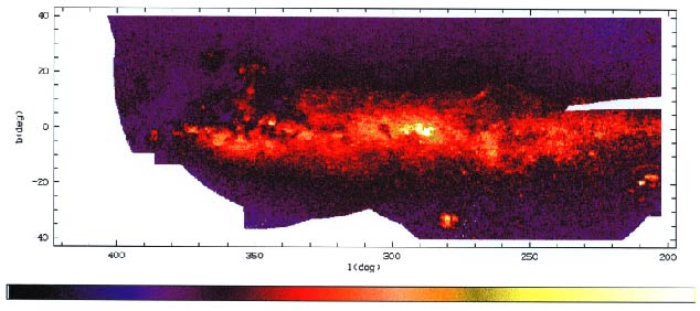
Figure 63: U photometry of the Southern Milky Way. The photometry is accompanied by a colour bar. Its left end corresponds to . The brightness at the right end of the bar is 450 S₁₀ units (U). The scale is linear. White areas denote non-valid data

  
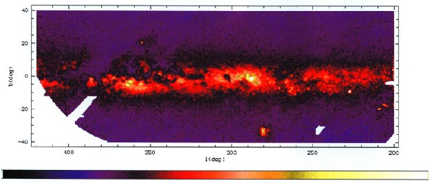
Figure 64: B photometry of the Southern Milky Way. The photometry is accompanied by a colour bar. Its left end corresponds to . The brightness at the right end of the bar is 550 S₁₀ units (B). The scale is linear. White areas denote non-valid data

  
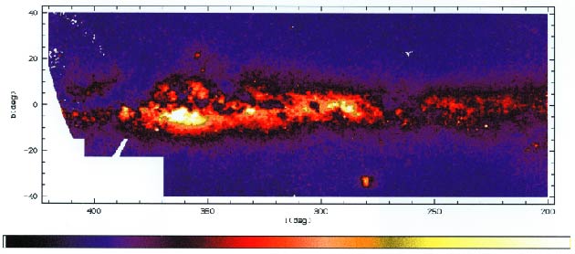
Figure 65: V photometry of the Southern Milky Way. The photometry is accompanied by a colour bar. Its left end corresponds to . The brightness at the right end of the bar is 900 S₁₀ units (V). The scale is linear. White areas denote non-valid data

  
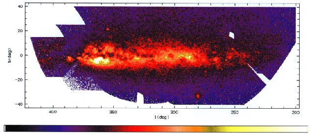
Figure 66: R photometry of the Southern Milky Way. The photometry is accompanied by a colour bar. Its left end corresponds to . The brightness at the right end of the bar is 2600 S₁₀ units (R). The scale is linear. White areas denote non-valid data

  
Figure 67: Synopsis of the Carina-Coalsack region in U, B, V, R. To facilitate comparison, the levels are adjusted for an optimal visualization. The S₁₀-isophotes in the sense of "outer broken line, continuous line and inner broken line" are (150, 250, 380) for U, (150, 230, 400) for B, (250, 500, 800) for V, and (1000, 1400, 1900) for R. The linear scale of the colour coding may be used for interpolation

   

Leinert & Richter (1981) =

Pröll (1980) =

Pfleiderer & Mayer (1971) =

Seidensticker et al. (1982) = B passband

Classen (1976) =

Leinert & Richter (1981) =

Mattila (1973) =

Seidensticker et al. (1982) =

Toller (1990) = V passband

Dachs (1970) =

Elsässer & Haug (1960) =

Leinert & Richter (1981) =

Seidensticker et al. (1982) = R passband

Seidensticker et al. (1982) =

Table 32: Comparison of the Bochum UBVR photometries (denoted as "X") with other photometries

10.4. Pioneer 10/11 spaceborne visual photometry

Small imaging photopolarimeters (IPP's) on the Pioneer 10 and 11 deep space probes were used during cruise phases (between and beyond the planets) to periodically measure and map over the sky brightness and polarisation in blue () and red () bands. This was done at heliocentric distances beyond 1.015 AU (Weinberg et al. 1974; Hanner et al. 1974). Early results suggested that observations of the same sky regions decreased in brightness with heliocentric distance R to 3.3 AU (Weinberg et al. 1974; Hanner et al. 1976), beyond which there was no observable change; i.e., the zodiacal light became vanishingly small compared to the background galactic light (i.e. was less than 2 ). Subsequent analysis (Schuerman et al. 1977) found this detectability limit to be 2.8 AU. Thus, for sky maps made between 1 AU and 2.8 AU, the observations give the sum of zodiacal light and background starlight, while beyond 2.8 AU the background starlight, including some diffuse galactic light, could be observed directly. We summarise here those observations from beyond 2.8 AU.

Approximately 80 sky maps were obtained with the Pioneer 10 IPP, starting in March 1972, of which 50 maps fall into the year 1972 (see Table 33 (click here)). The FOV's covered most of the sky (see Fig. 68 (click here)) except for a region near the spin axis of the spacecraft (within 30 of the sun). Table 33 (click here) presents a log of observations with the Pioneer 10 IPP. A similar schedule was performed with the IPP on Pioneer 11, starting in April 1973. The combined data provide a higher spatial resolution than would have been possible to obtain with a single map or with observations from a single spacecraft (S/C). Further, Pioneer 11 obtained 12 additional maps between November 1981 and December 1982 to "fill in" the aforementioned sky gap regions.

The instantaneous field of view of each IPP was approximately 2.3 square. Brightness was integrated for 1/64 (one sector) of the 12.5 s spacecraft spin period, giving a maximum effective FOV of when the telescope was perpendicular to the spin axis (). The spin axis was directed more or less toward the sun. By moving the IPP telescope in steps of 1.8 in look angle, the entire sky between 29 and 170 from the spin axis could be scanned. The spinning, sectoring and stepping resulted in a two-dimensional overlapping pattern of FOV's on the sky for each map (see Fig. 68 (click here)). Since the spin axis moved slowly on the celestial sphere according to the moving spacecraft position, most of the sky was eventually covered with a resolution better than the 1.8 roll-to-roll separation of FOV's in a single map.

  
Figure 68: Example for Pioneer data in the blue (440 nm), from a sky map observed beyond 3 AU. Upper panel: Map of the Becvar atlas showing part of the southern Milky Way and the Magellanic clouds, with the sectored field-of-view of Pioneer 10 overlaid. Middle panel: Brightness values in units interpolated from the individual sector brightnesses to a rectangular coordinate grid. Lower panel: Isocontour map constructed from this set of brightnesses

   

Year Calendar Sun-S/C S/C Distance Heliocentric Usable LA^b Signal/

Date Distance from ecliptic^a Range Noise

(AU) (AU) (deg) (deg)

1972 Mar. 10 1.002 -.0065 -0.37 172.85 152-168 8.70

11 1.004 -.0073 -0.41 174.12 135-167 4.15

12 1.006 -.00805 -0.46 175.36 136-169 7.68

14 1.011 -.0095 -0.54 177.63 128-169 7.00

15 1.014 -.0103 -0.58 178.87 128-168 5.65

16 1.017 -.01107 -0.62 180.07 128-169 4.93

20 1.032 -.01428 -0.79 185.03 128-150 5.62

22 1.040 -.01581 -0.87 187.37 128-168 5.00

23 1.046 -.01677 -0.92 188.84 128-170 4.56

29 1.075 -.02117 -1.13 195.47 128-169 6.43

31 1.087 -.0227 -1.20 197.78 110-146 5.87

Apr. 4 1.110 -.02554 -1.32 201.95 110-170 4.93

10 1.150 -.02971 -1.48 207.98 91-159 4.12

13 1.171 -.03165 -1.55 210.76 91-170 3.78

17 1.201 -.03424 -1.63 214.39 91-166 3.15

20 1.224 -.03613 -1.69 217.02 91-168 4.71

27 1.281 -.04027 -1.80 222.68 86-103 4.09

28 1.289 -.04086 -1.82 223.48 91-158 3.75

May 5 1.349 -.04474 -1.90 228.64 46-168 11.46

8 1.376 -.04632 -1.93 230.73 46-156 14.43

17 1.453 -.05058 -1.99 236.23 46-170 13.87

30 1.586 -.05694 -2.06 244.26 46-169 10.34

June 7 1.652 -.05972 -2.07 247.70 46-169 8.90

13 1.709 -.06196 -2.08 250.46 49-130 7.75

20 1.774 -.06436 -2.08 253.40 42-067 7.96

22 1.788 -.06485 -2.08 254.00 44-170 7.31

27 1.841 -.06666 -2.08 256.21 91-130 4.21 141-168

29 1.861 -.0673 -2.07 257.00 68-169 5.21

July 21 2.062 -.07326 -2.04 264.32 128 3.87

24 2.090 -.07399 -2.03 265.22 128 6.40

27 2.117 -.07469 -2.02 266.11 128 4.34

31 2.152 -.07557 -2.01 267.21 128 7.75

Aug. 3 2.179 -.07622 -2.00 268.04 104-137 4.81 160-170

10 2.241 -.07766 -1.99 269.87 128 5.00

11 2.249 -.07784 -1.98 270.11 91-140 4.43 158-170

16 2.294 -.07880 -1.97 271.36 91-168 6.31

23 2.354 -.08005 -1.95 273.01 74-145 5.90 167-170

30 2.413 -.08121 -1.93 274.58 76-158 4.03

Sept. 5 2.467 -.08219 -1.91 275.94 76-166 5.09

8 2.492 -.08263 -1.90 276.56 128-169 4.59

26 2.640 -.085005 -1.85 280.07 76-105

27 2.641 -.08502 -1.84 280.09 76-150 7.34

Oct. 10 2.750 -.08652 -1.80 282.50 49-79 5.15

Oct. 18 2.812 -.08728 -1.78 283.81 (42-68)^* 4.78 (77-163)^*

19 2.821 -.08739 -1.78 283.99 (91-157)^* 4.71

Nov. 4 2.939 -.08865 -1.73 286.37 42-161 4.93

19 3.056 -.08969 -1.68 288.63 43-173 2.62

Dec. 4 3.163 -.09046 -1.64 290.61 42-170 2.90

19 3.269 -.09104 -1.60 292.47 40-170 5.15

Table 33: Log of cruise phase observations with the Pioneer 10 imaging photopolarimeter

 

Year Calendar Sun-S/C S/C Distance Heliocentric Usable LA^b Signal/

Date Distance from ecliptic^a Range Noise

(AU) (AU) (deg) (deg)

1973 Jan. 5 3.384 -.09150 -1.55 294.44 38-115 3.50

8 3.404 -.09155 -1.54 294.77 109-163 2.71

Feb. 1 3.560 -.09180 -1.48 297.32 67-144 4.96

13 3.805 -.09146 -1.38 301.10 (152-170)^* 5.59

Mar. 3 3.927 -.09095 -1.33 302.92 128-137 4.21 148-170

28 4.065 -.09009 -1.27 304.92 91-128 6.68 154-170

May 29 4.226 -.08868 -1.20 307.21 38-170 6.71

June 7 4.273 -.08818 -1.18 307.88 91-121 6.59

Aug. 4 4.545 -.08449 -1.07 311.66 91-170 5.53

6 4.553 -.08434 -1.06 311.78 38- 94 4.96

25 4.636 -.08289 -1.02 312.92 38-145 6.31

Oct. 6 4.812 -.07924 -0.94 315.34 38-148 5.12 164-169

26 4.892 -.07730 -0.91 316.41 38-115 5.53 128-170

1974 Jan. 21 5.084 -.03264 -0.36 325.43 38-170 4.18

Mar. 9 5.152 -.00128 0.00 332.08 38-170 4.15

Apr. 21 5.253 +.03021 +0.33 338.05 38-109 4.06

22 5.254 +.03033 +0.33 338.07 111-170 4.46

June 25 5.466 +.07531 +0.79 346.36 40-152 4.34 168-170

Aug. 31 5.748 +.12004 +1.20 354.15 38-170 5.18

Oct. 28 6.042 +.15838 +1.50 0.31 38-168 12.40

1975 Jan. 28 6.576 +.21749 +1.90 8.83 47- 77 3.90 100 147-167

Mar. 28 6.953 +.25429 +2.10 13.57 42-91 3.09 103-170

May 21 7.137 +.28729 +2.25 17.47 109-170 4.81

30 7.378 +.29265 +2.27 18.07 37-114 4.46 124-132 143-170

July 27 7.787 +.32721 +2.41 21.77 46-152 4.21

Sept. 30 8.261 +.36524 +2.53 25.49 35-168 5.25

Nov. 28 8.704 +.39919 +2.63 28.53 35- 68 3.06 94-109 122-126 135-169

1976 Jan. 30 9.182 +.43440 +2.71 31.41 42-127 2.40 135-170

^apositive values mean a location of the spacecraft north of the ecliptic plane.
^bLA = look angle = angle measured from the spin axis.
^*Approximately 1/2 of the data are lost due to low data rate and other factors.

The data reduction methodology is described in a User's Guide (Weinberg & Schuerman 1981) for the Pioneer 10 and Pioneer 11 IPP data archived at the National Space Science Data Center (NSSDC). Signals of bright stars were used to calibrate the decaying sensitivity of the IPP channels. Individually resolved stars, typically those brighter than 6.5 mag, were removed from the measured brightnesses on the basis of a custom made catalog containing 12457 stars. The absolute calibration was based on the instrument's response to Vega. Finally, the Pioneer 10 and 11 blue and red data were represented in units. The result is a background sky tape, which, for the data beyond 2.8 AU, contains the integrated starlight, including the contribution from the diffuse galactic light. A more complete description of the reduction and use of the data is being prepared (Weinberg, Toller, and Gordon). The data can be accessed under http://nssdc.gsfc.nasa.gov/, following from there on the topics "Master catalog", "Pioneer 10" and "Experiment information".

The background sky data set can be addressed in a variety of ways, including overlaying the data on a sky atlas such as Becvar's Atlas Coeli (1962), interpolating the posted data on an evenly spaced coordinate grid, and contouring the data. Each of these is shown in the three panels of Fig. 68 (click here), all covering the south celestial pole region, which includes low galactic latitude regions and both the Small and Large Magellanic Clouds. The map scale and magnitude limit of the Atlas Coeli make this atlas convenient for illustrating and manipulating Pioneer background sky data. The upper panel in Fig. 68 (click here) shows a single Pioneer 10 map's pattern of FOV's overlaid on the corresponding region of the Becvar atlas. The map shows the overlap in both look angle and sector (day 68 of year 1974, observed at R=5.15 AU). The middle panel shows the result of interpolating the data for six map days of observations in blue on an evenly spaced coordinate grid for the same region of sky. We estimate that the random error in the numbers shown in the middle panel is 2 to 3 units, and perhaps 5 units in the Milky Way and the Magellanic clouds. An isophote representation of the data (lower panel) is perhaps the most convenient way to present the data. The interval between isophotes is 5 units. The spatial resolution was found to be approximately 2. Regularly spaced grid values of Pioneer 10 blue and red brightnesses were determined in this manner for the entire sky, from which data were derived every two degrees both in galactic and equatorial coordinates. Part of these data are used in Tables 35 to 38 to depict Pioneer 10 blue and red data at 10 intervals in both coordinate systems. Pioneer 11 data showed no significant differences to Pioneer 10 data, so only Pioneer 10 data are discussed and shown here.

More recently, Gordon (1997) further analyzed Pioneer 10 and 11 data from beyond the asteroid belt. He also found no significant differences between the Pioneer 10 and 11 data. His grey scale presentation of the combined data with 0.5 spatial resolution is shown in an Aitoff projection in Fig. 69 (click here). The gap in this figure corresponds to that discussed earlier. Gordon did not have available those special data sets closing the gap.

  
Figure 69: Pioneer 10/11 blue sky map at 440 nm at 0.5 resolution, constructed from Pioneer 10 and Pioneer 11 maps taken at 3.26 AU to 5.15 AU heliocentric distance. The map is in Aitoff projection. The galactic center is at the center. From Gordon (1997)

From the Pioneer data, blue and red brightnesses at the celestial, ecliptic and galactic poles were derived from isophote maps of the polar regions like the one shown for the south celestial pole in Fig. 68 (click here). They are compared with other photometric data and with star counts in Table 34 (click here). There is fair agreement among the photometries. However, because of the lack of atmospheric and interplanetary signals in the Pioneer data, these data should be preferred over the other photometries when determining the level of galactic light in a certain region. Generally the photometries are at higher levels than the star counts, as one would expect, since the photometries contain the contributions of diffuse galactic light (Sect. 11 (click here)) and extragalactic background light (Sect. 12 (click here)). Equal numbers for the brightnesses in the blue and the red shown in Table 34 (click here) would mean that the galactic component of the night sky brightness has solar colour. The Pioneer data show a reddening at the poles, and this reddening appears all over the sky (see Tables 35- 38). Details can be found in Toller (1981) and Toller (1990).

   

Wavelength 4250 4400 Blue Red

(Å) 4150 6440

(Year) et al. 10 & Haug (1968) (1976) et al. Megill Lipaeva (1973) (1973) 10

1997 (1978) (1960) 1993 (1961) (1973) (1978)

NEP 66 <95 98 52 50 66 76 82

NGP 29 27 22 24 21 26 41 31

SCP 52 86 74 <95 58 55 56 41 94

SEP 61 106 128 124 87 67 50 39 125

SGP 26 33 27 28 23 53 79 36

Table 34: Brightnesses of background starlight and integrated starlight at the north and south celestial, ecliptic, and galactic poles (in units). Stars with m_V < 6.5 excluded. Adapted from Toller et al. (1987)

   
Table 35: Pioneer 10 background starlight in blue (440 nm), given in galactic coordinates and units. From Toller (1981)

   
Table 36: Pioneer 10 background starlight in red (640 nm), given in galactic coordinates and units. From Toller (1981)

   
Table 37: Pioneer 10 background starlight in blue (440 nm), in equatorial coordinates and units. From Toller (1981)

   
Table 38: Pioneer 10 background starlight in red (640 nm), in equatorial coordinates and units. From Toller (1981)

  
Figure 70: Comparison of Pioneer 10 data for cuts through the Milky Way at different longitudes with the results of other investigations. Note that the ordinate is in S₁₀(B) units. The numbers given in Table 35 (click here), which are given in units, are therefore larger by a factor corresponding to the solar B-V value (compare Table 2)

Pioneer blue data are compared in Fig. 70 (click here) to star counts and some earthbased photometric observations along four cuts through the Milky Way at different galactic longitudes. Generally, Classen's (1976) results agree quite well with the Pioneer data, also at high galactic latitudes, except at and at middle latitudes where they are much lower, possibly from errors in the difficult corrections for airglow and atmospheric extinction, since her observations of this region had to be made near the horizon (from South Africa). Generally speaking, all ground-based data sets suffer from the presence of airglow continuum and some from line emission (see Sect. 6 (click here)) in the instrument's spectral band (see Weinberg & Mann 1967). However, ground-based photometries may offer better spatial resolution, like the Bochum Milky Way photometries presented in Sect. 10.3 above, and these particular photometries also give realistic absolute brightness values, as judged from their good agreement with the Helios U, B, V photometry.

10.5. Near- and mid-infrared

Maps of the starlight distribution in the infrared are difficult to obtain. There are currently no sensitive, all-sky surveys of stars in the infrared, though the ground-based 2MASS and DENIS programs will provide that in the next several years. Extracting starlight maps from diffuse sky brightness measurements is challenging because of the need to separate the various contributions to the measured light. The COBE/DIRBE team has developed a detailed zodiacal light model which allows such a separation, at least in the near-infrared.

An all-sky image dominated by the stellar light of the Galaxy is presented in Fig. 71 (click here). The map was prepared by averaging 10 months of DIRBE data at 2.2 m wavelength after removal of the time-dependent signal from solar-system dust via a zodiacal light model. The remaining sky brightness at this wavelength is dominated by the cumulative light from K and M giants (Arendt et al. 1994), though individual bright sources can be detected at a level of about 15 Jy above the local background in unconfused regions. Although this map also contains small contributions from starlight scattered by interstellar dust (cirrus) and any extragalactic emission, these contributions are much smaller than that from stars. No extinction correction has been applied to the map in Fig. 71 (click here); Arendt et al. (1994) found 2.2 m optical depths greater than 1 within 3 of the Galactic plane for directions toward the inner Galaxy and bulge (|l| < 70). Arendt et al. used the multi-wavelength DIRBE maps to construct an extinction-corrected map over the central part of the Milky Way.

The typical appearance of the galactic stellar emission in the infrared the Milky Way is apparent in Fig. 71 (click here): because the interstellar extinction is much reduced in the infrared, this internal view of our Galaxy looks like a galaxy seen edge-on from the outside. Bulge and disk are clearly visible and separated. This appearance shows at all near-infrared wavelengths (see Fig. 72 (click here)).

  
Figure 71: DIRBE map of sky brightness at 2.2 microns in galactic coordinates, with zodiacal light removed. North is up, the galactic center in the middle, and galactic longitude increasing from right to left. This map is dominated by galactic starlight. No extinction correction has been made. Intensities are provided at 16 levels on a logarithmic scale ranging from 0.04 to 32 MJy/sr. In detail these levels are: 0.040, 0.062, 0.097, 0.15, 0.24, 0.37, 0.57, 0.90, 1.40, 2.19, 3.41, 5.33, 8.32, 12.98, 20.26, and 31.62 MJy/sr

  
Figure 72: DIRBE maps of sky brightness at 1.25, 2.2, 3.5, and 4.9 m at low Galactic latitudes ( within 30 degrees of Galactic center, and elsewhere). Zodiacal light has been removed. North is up, and galactic longitude is increasing from right to left. These maps are generally dominated by Galactic starlight. No extinction correction has been made. Intensities are provided at 16 levels on logarithmic scales ranging from 0.6 to 25 MJy/sr (1.25 m and 2.2 m), 0.4 to 16 MJy/sr (3.5 m), and 0.3 to 12.5 MJy/sr (4.9 m). In detail these levels are: 0.63, 0.81, 1.03, 1.32, 1.69, 2.15, 2.75, 3.52, 4.50, 5.75, 7.36, 9.40, 12.02, 15.37, 19.65, and 25.12 MJy/sr at 1.25 m and 2.2 m; 0.40, 0.51, 0.65, 0.83, 1.06, 1.36, 1.74, 2.22, 2.84, 3.63, 4.64, 5.93, 7.59, 9.70, 12.40, and 15.85 MJy/sr at 3.5 m; 0.32, 0.40, 0.52, 0.66, 0.84, 1.08, 1.38, 1.76, 2.26, 2.88, 3.69, 4.71, 6.03, 7.70, 9.85, and 12.59 MJy/sr at 4.9 m

  
Figure 73: Intensity profiles of "Galactic starlight" as measured from the DIRBE maps at 1.25 m, 2.2 m, 3.5 m and 4.9 m after subtraction of zodiacal light. Upper half: longitudinal profiles at a fixed Galactic latitude of ( is not shown as representative because extinction is significant at some wavelengths). Lower half: latitudinal profiles at fixed Galactic longitude of

  
Figure 74: Residual contributions to the near-infrared background radiation of stars fainter than a given apparent magnitude, for galactic latitudes of 20, 50, and 90 (from top to bottom, respectively). The values at the galactic pole at the intersection with the ordinate axis (cutoff magnitude = 3 mag) corresponds to 0.063 MJy/sr for J, to 0.081 MJy/sr for K, and to 0.053 MJy/sr for the L waveband

To look at the starlight distribution over a broader spectral range, it is useful to concentrate on the low Galactic-latitude region. Figure 72 (click here) presents DIRBE maps of this region at 1.25 m, 2.2 m, 3.5 m and , each with the zodiacal light removed using the DIRBE zodiacal light model. Since starlight is the dominant source at low latitudes over this spectral range, these maps are a good approximation to the infrared stellar light, with extinction of course decreasing as wavelength increases. Corresponding maps at 12 microns and longer are not shown, because at these wavelengths interplanetary dust emission becomes the dominant contributor to sky brightness, and artifacts from imperfect removal of the zodiacal emission become more serious, as does the contribution from cirrus cloud emission. More elaborate modeling would be required to extract the stellar component of the sky brightness at these wavelengths. Figure 73 (click here) shows two sets of repesentative intensity profiles taken from the 1.25 m - 4.9 m approximate "starlight" maps: the first set on a constant-latitude line near the Galactic plane and the second along the zero-longitude meridian. Full-sky DIRBE maps at 1.25 m, 2.2 m, 3.5 m, 4.9 m, 12 m, 25 m, 60 m, 100 m, 140 m, and 240 m with the zodiacal light removed, from which these approximate starlight maps have been selected, are available as the "Zodi-Subtracted Mission Average (ZSMA)" COBE data product, available from the NSSDC through the COBE homepage website at http://www.gsfc.nasa.gov/aas/cobe/cobe_-home.html.

Model predictions for the integrated starlight, based on the galaxy model of Bahcall & Soneira (1980), were given for the near- and mid-infrared as function of the brightness of the individually excluded stars by Franceschini et al. (1991b). Figures 74 (click here) and 75 (click here) show these results for wavelengths of 1.2 m, 2.2 m, 3.6 m, and 12 m.

  
Figure 75: Residual contributions to the 12 m background radiation of stars fainter than a given flux limit, for galactic latitudes of 20, 50, and 90 (from top to bottom, respectively). The values at the galactic pole at the intersection with the ordinate axis (cutoff flux = 20 Jy) correspond to 0.002 MJy/sr, which is much less than the contribution due to diffuse emission from the interstellar medium