We have shown that our radiation hydrodynamics code is capable of finding
steady state solutions for stellar outflows driven by radiation pressure on
dust for a wide variety of stellar parameters and mass loss rates.
We have checked that the code finds the correct solution for the case of gray
dust opacities and no drift velocity, for which an analytical solution is
easily obtained. Numerical errors of the order ![]() (
(![]() :
numerical resolution of the radial grid) are kept below
:
numerical resolution of the radial grid) are kept below ![]() by a
proper choice of the radial grid.
by a
proper choice of the radial grid.
For more realistic cases with non-gray dust opacities and including drift of
dust relative to gas, we compared our results with those published by Netzer
& Elitzur (1993). For Oxygen stars we notice that neither the shape of the
relation ![]() (
(![]() ) nor the values of the terminal gas velocities
) nor the values of the terminal gas velocities ![]() \
(except for the lowest mass loss rates) are in reasonable agreement, in some
cases differing by a factor of 2. While all of our models show a maximum
outflow velocity at intermediate mass loss rates (
\
(except for the lowest mass loss rates) are in reasonable agreement, in some
cases differing by a factor of 2. While all of our models show a maximum
outflow velocity at intermediate mass loss rates (![]()
![]()
![]() /yr) and a distinct decrease of
/yr) and a distinct decrease of ![]() towards higher mass loss rates, the
models of NE exhibit a monotonic increase of
towards higher mass loss rates, the
models of NE exhibit a monotonic increase of ![]() with mass loss rate.
Although NE give an explanation for this behavior, we believe that our models
are more appropriate. Qualitatively, our results for Oxygen stars are confirmed
by the work of Habing et al. (1995).
with mass loss rate.
Although NE give an explanation for this behavior, we believe that our models
are more appropriate. Qualitatively, our results for Oxygen stars are confirmed
by the work of Habing et al. (1995).
We have tried to identify the reason for this discrepancy with respect to NE. For instance, we have checked that the gravitational force of the shell itself, which is included in our code but is ignored by NE, is no explanation. For a few examples, we have investigated the effect of arbitrarily changing the absorption cross section by 20% at all wavelengths. We conclude that uncertainties of this magnitude are not sufficient to bring our results into agreement with NE. Moreover, we checked that the opacities for astronomical silicates and graphite computed on the basis of Mie theory from the dielectric constants given by Draine (1987) (used by NE) are in excellent agreement with the opacities used in the present work. Test calculations suggest that certain approximations in the treatment of radiative transfer adopted by NE, in particular the Adams & Shu (1986) closure relation applied frequency by frequency, may lead to large errors in the case of optically thick dust shells. For some reason, this effect seems to be more pronounced for silicate dust. Another difference is that our radiative transfer scheme resolves the central star while NE treat it as a point source, which may be a questionable approximation.
In addition, we have checked our code against a completely independent radiative transfer code (DUSTCD, cf. Leung 1975, 1976; Egan et al. 1978) suitable for the computation of the infrared radiation field of dusty stellar envelopes. In all cases investigated (optically thin and optically thick winds, gray opacities) we found excellent agreement. Note that in order to achieve a reasonable energy conservation with DUSTCD, a sufficient spatial resolution in the acceleration region of the shell was found to be essential.
Finally we would like to point out that our test calculations have clearly
demonstrated that, in general, gas pressure cannot be neglected in the equation
of motion. Our results show that in practice gas pressure is important unless
the terminal outlow velocities are really highly supersonic, i.e.
![]() . For slow AGB winds (
. For slow AGB winds (![]() km/s), the outflow
velocities may become up to 50% larger (cf. Figs. 15 (click here) to
17 (click here)) if gas pressure is allowed to support the wind. These conclusions
are based on the assumption that
km/s), the outflow
velocities may become up to 50% larger (cf. Figs. 15 (click here) to
17 (click here)) if gas pressure is allowed to support the wind. These conclusions
are based on the assumption that ![]() and a mean
molecular weight of the gas of
and a mean
molecular weight of the gas of ![]() . Actually,
. Actually, ![]() ,
corresponding to hydrogen in molecular form, may be more appropriate and
would reduce the importance of gas pressure roughly by a factor of two. On
the other hand, T may actually be higher than
,
corresponding to hydrogen in molecular form, may be more appropriate and
would reduce the importance of gas pressure roughly by a factor of two. On
the other hand, T may actually be higher than ![]() \
due to frictional heating (Krüger et al. 1994), leading to a corresponding
enhancement of the role of gas pressure, especially in the case of large
drift velocity, i.e. low mass loss rates (Kastner 1992).
\
due to frictional heating (Krüger et al. 1994), leading to a corresponding
enhancement of the role of gas pressure, especially in the case of large
drift velocity, i.e. low mass loss rates (Kastner 1992).
Along with the hydrodynamics of AGB winds, we have computed the emergent
spectral energy distribution (SED) of the star plus circumstellar dust shell.
From the analysis of this sample of spectra we infer that, for fixed dust
properties, all models fall on a simple color-color relation in the IRAS
two-color-diagrams, with ![]() (or optical depth) being the only parameter.
(or optical depth) being the only parameter.
Surprisingly, we found a close agreement between the synthetic spectra resulting from the self-consistent hydrodynamical approach and those obtained from much simpler models based on a constant outflow velocity and ignoring dust drift. Obviously, the effects of assuming a constant outflow velocity and neglecting the dust drift velocity cancel to some degree. We conclude that ``simple'' models may be used for the analysis of observed SEDs without introducing large systematic errors, provided the adopted constant outflow velocity equals the observed one.
This study constitutes the basis for future time-dependent hydrodynamical calculations. In a subsequent paper we will investigate the dynamical response of circumstellar gas/dust shells to the temporal variations of the stellar parameters and mass loss rate. To our knowledge, this problem has not yet been addressed by real radiation hydrodynamics calculations, although it is well known that the stellar parameters and the mass loss rate can undergo significant variations on rather short time scales when intermediate mass stars experience so called ``thermal pulses'' on the upper AGB.
Acknowledgements
This research has been funded by ``Deutsche Agentur für Raumfahrtangelegenheiten'' (DARA) under grant 50 OR 9411. One of us (R. Sz.) expresses his gratitude to the Canadian Institute of Theoretical Astrophysics and to the Polish State Committee for Scientific Research - grant No. 2.P03D.027.10. A.M. and R.Sz. are grateful for the hospitality and support provided by the Astrophysical Institute Potsdam. We are indebted to H. Yorke for the permission to modify his original code and to apply it to the problem of dusty stellar outflows.

Figure 2:
Model results for an Oxygen star with ![]()
![]() ,
, ![]()
![]() , and
, and ![]() K for 3 different mass loss rates (indicated in the title
of each panel). The dust is assumed to consist of grains of astronomical
silicates with properties given in Table 1 (click here). The initial velocity at
the dust formation point is assumed to be u1 = 2 km/s. The left hand panels
show the gas velocity (solid) and the dust velocity (dashed) as a function of
radial distance. The right hand panels show the corresponding stellar input
spectrum (dot-dashed) and the emergent spectral energy distribution (solid)
which is the result of processing of the stellar radiation by the dusty
envelope. More information about these models (C6_m, C3_m, C1_m) and
additional runs of this sequence is listed in Table 2
K for 3 different mass loss rates (indicated in the title
of each panel). The dust is assumed to consist of grains of astronomical
silicates with properties given in Table 1 (click here). The initial velocity at
the dust formation point is assumed to be u1 = 2 km/s. The left hand panels
show the gas velocity (solid) and the dust velocity (dashed) as a function of
radial distance. The right hand panels show the corresponding stellar input
spectrum (dot-dashed) and the emergent spectral energy distribution (solid)
which is the result of processing of the stellar radiation by the dusty
envelope. More information about these models (C6_m, C3_m, C1_m) and
additional runs of this sequence is listed in Table 2

Figure 3:
Same as Fig. 2 (click here) but for an Oxygen star with ![]()
![]() ,
,
![]()
![]() , and
, and ![]() K
(note that the range of mass loss rates and
the scaling of the plots is different). As in the previous sequence
(Fig. 2 (click here)) the initial velocity at the dust formation point is u1 =
2 km/s. More information about these models (D5_m, D3_m, D1_m) and
additional runs of this sequence is listed in Table 3. The dotted
spectral energy distribution was computed from a simplified model, assuming a
constant velocity,
K
(note that the range of mass loss rates and
the scaling of the plots is different). As in the previous sequence
(Fig. 2 (click here)) the initial velocity at the dust formation point is u1 =
2 km/s. More information about these models (D5_m, D3_m, D1_m) and
additional runs of this sequence is listed in Table 3. The dotted
spectral energy distribution was computed from a simplified model, assuming a
constant velocity, ![]() , where
, where ![]() is the terminal gas outflow velocity
obtained from the hydrodynamical model with the same parameters
is the terminal gas outflow velocity
obtained from the hydrodynamical model with the same parameters

Figure 4:
Same as Fig. 2 (click here) but for an Oxygen star with ![]()
![]() ,
,
![]()
![]() , and
, and ![]() K. The initial velocity at
the dust formation point is u1 = 4 km/s.
More information about these models (E5_m, E3_m, E1_m) and additional runs
of this sequence is listed in Table 4
K. The initial velocity at
the dust formation point is u1 = 4 km/s.
More information about these models (E5_m, E3_m, E1_m) and additional runs
of this sequence is listed in Table 4

Figure 5:
Same as Fig. 2 (click here) but for an Oxygen star with ![]()
![]() ,
,
![]()
![]() , and
, and ![]() K. As in the previous
sequence (Fig. 4 (click here)) the initial velocity at the dust formation point
is u1 = 4 km/s.
More information about these models (F4_m, F2_m, F1_m) and additional runs
of this sequence is listed in Table 5
K. As in the previous
sequence (Fig. 4 (click here)) the initial velocity at the dust formation point
is u1 = 4 km/s.
More information about these models (F4_m, F2_m, F1_m) and additional runs
of this sequence is listed in Table 5

Figure 6:
Model results for a Carbon star with ![]()
![]() ,
,
![]()
![]() , and
, and ![]() K for 3 different mass loss
rates (indicated in the heading of each panel). The dust is assumed to
consist of grains of graphite with properties given in
Table 1 (click here). The initial velocity at the dust formation point is assumed
to be u1 = 2 km/s. The left hand panels show the gas velocity (solid) and
the dust velocity (dashed) as a function of radial distance.
The right hand panels show the corresponding stellar input spectrum (dot-dashed)
and the emergent spectral energy distribution (solid) which is the result of
processing of the stellar radiation by the dusty envelope.
More information about these models (G6_m, G3_m, G1_m) and additional runs
of this sequence is listed in Table 6. The dotted spectral energy
distribution was computed from a simplified model, assuming a constant
velocity,
K for 3 different mass loss
rates (indicated in the heading of each panel). The dust is assumed to
consist of grains of graphite with properties given in
Table 1 (click here). The initial velocity at the dust formation point is assumed
to be u1 = 2 km/s. The left hand panels show the gas velocity (solid) and
the dust velocity (dashed) as a function of radial distance.
The right hand panels show the corresponding stellar input spectrum (dot-dashed)
and the emergent spectral energy distribution (solid) which is the result of
processing of the stellar radiation by the dusty envelope.
More information about these models (G6_m, G3_m, G1_m) and additional runs
of this sequence is listed in Table 6. The dotted spectral energy
distribution was computed from a simplified model, assuming a constant
velocity, ![]() , where
, where ![]() is the terminal gas outflow velocity obtained
from the hydrodynamical model with the same parameters
is the terminal gas outflow velocity obtained
from the hydrodynamical model with the same parameters
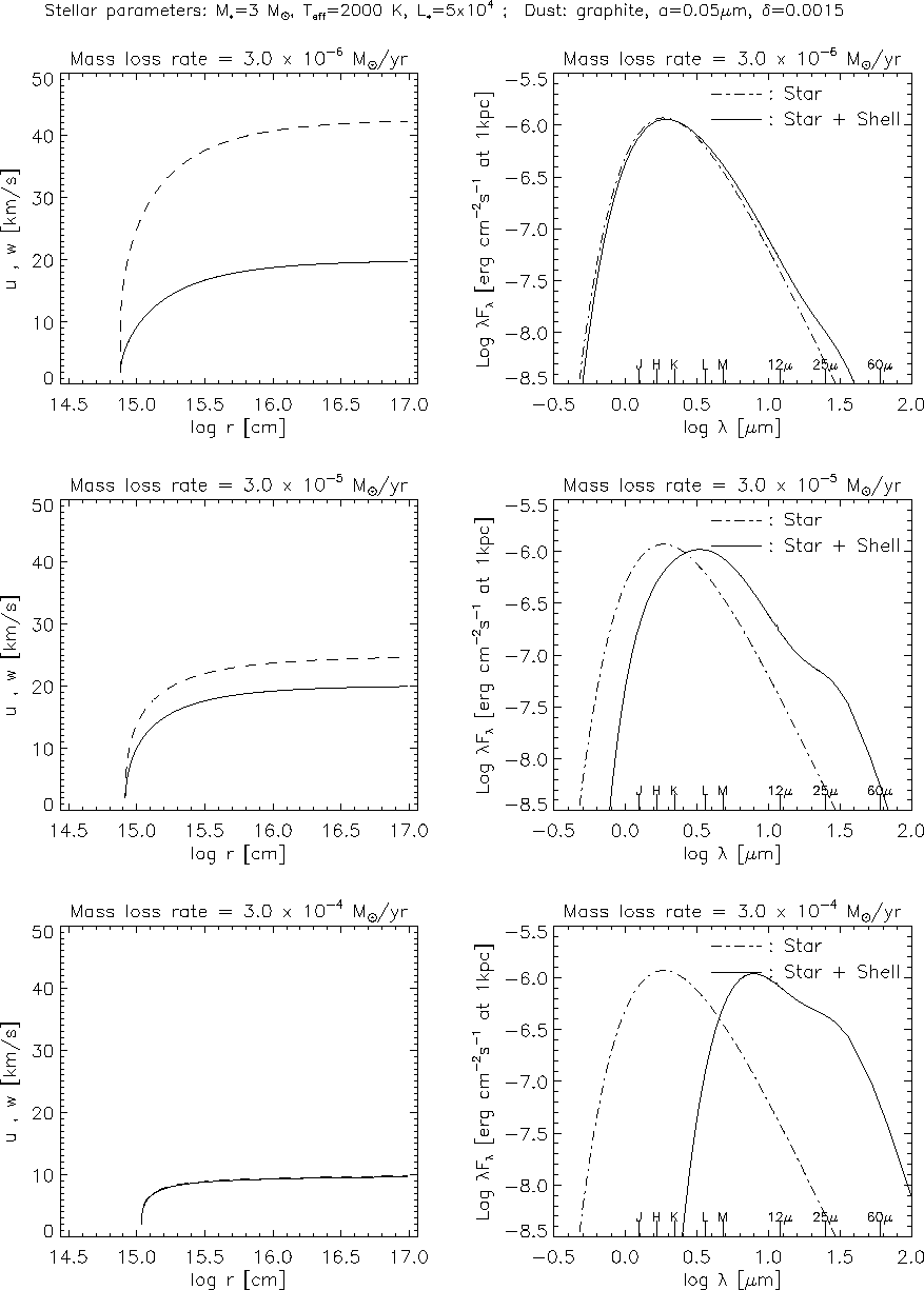
Figure 7:
Same as Fig. 6 (click here) but for a Carbon star with ![]()
![]() ,
,
![]()
![]() , and
, and ![]() K (note that the range of mass
loss rates and the scaling of the plots is different).
More information about these models (H6_m, H4_m, H2_m) and additional runs
of this sequence is listed in Table 7
K (note that the range of mass
loss rates and the scaling of the plots is different).
More information about these models (H6_m, H4_m, H2_m) and additional runs
of this sequence is listed in Table 7

Figure 8:
Same as Fig. 6 (click here) but for a Carbon star with ![]()
![]() ,
,
![]()
![]() , and
, and ![]() K.
More information about these models (I5_m, I3_m, I1_m) and additional runs
of this sequence is listed in Table 8
K.
More information about these models (I5_m, I3_m, I1_m) and additional runs
of this sequence is listed in Table 8

Figure 9:
Same as Fig. 6 (click here) but for dust consisting of grains of amorphous
carbon with properties given in Table 1 (click here). More information about
these models (J6_m, J3_m, J1_m) and additional runs of this sequence is
listed in Table 9. The dotted spectral energy
distribution was computed from a simplified model, assuming a constant
velocity, ![]() , where
, where ![]() is the terminal gas outflow velocity obtained
from the hydrodynamical model with the same parameters
is the terminal gas outflow velocity obtained
from the hydrodynamical model with the same parameters

Figure 10:
Same as Fig. 9 (click here) but for a Carbon star with ![]()
![]() ,
,
![]()
![]() , and
, and ![]() K (note that the range of mass
loss rates and the scaling of the plots is different).
More information about these models (K6_m, K4_m, K2_m) and additional runs
of this sequence is listed in Table 10
K (note that the range of mass
loss rates and the scaling of the plots is different).
More information about these models (K6_m, K4_m, K2_m) and additional runs
of this sequence is listed in Table 10

Figure 11:
Same as Fig. 9 (click here) but for a Carbon star with ![]()
![]() ,
,
![]()
![]() , and
, and ![]() K.
More information about these models (L5_m, L3_m, L1_m) and additional runs
of this sequence is listed in Table 11
K.
More information about these models (L5_m, L3_m, L1_m) and additional runs
of this sequence is listed in Table 11
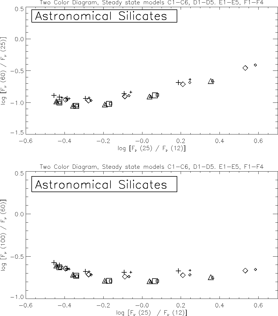
Figure 12:
Top: IRAS two-color diagram for the Oxygen star models C (+), D (![]() ),
E (
),
E (![]() ) and F (
) and F (![]() ). For each large symbol, indicating the position
of a model computed with gas pressure, there is a corresponding small symbol
close to it, showing the position of the respective model computed without
gas pressure. Bottom: Same as above, but showing the flux ratio
). For each large symbol, indicating the position
of a model computed with gas pressure, there is a corresponding small symbol
close to it, showing the position of the respective model computed without
gas pressure. Bottom: Same as above, but showing the flux ratio
![]() in the ordinate
in the ordinate
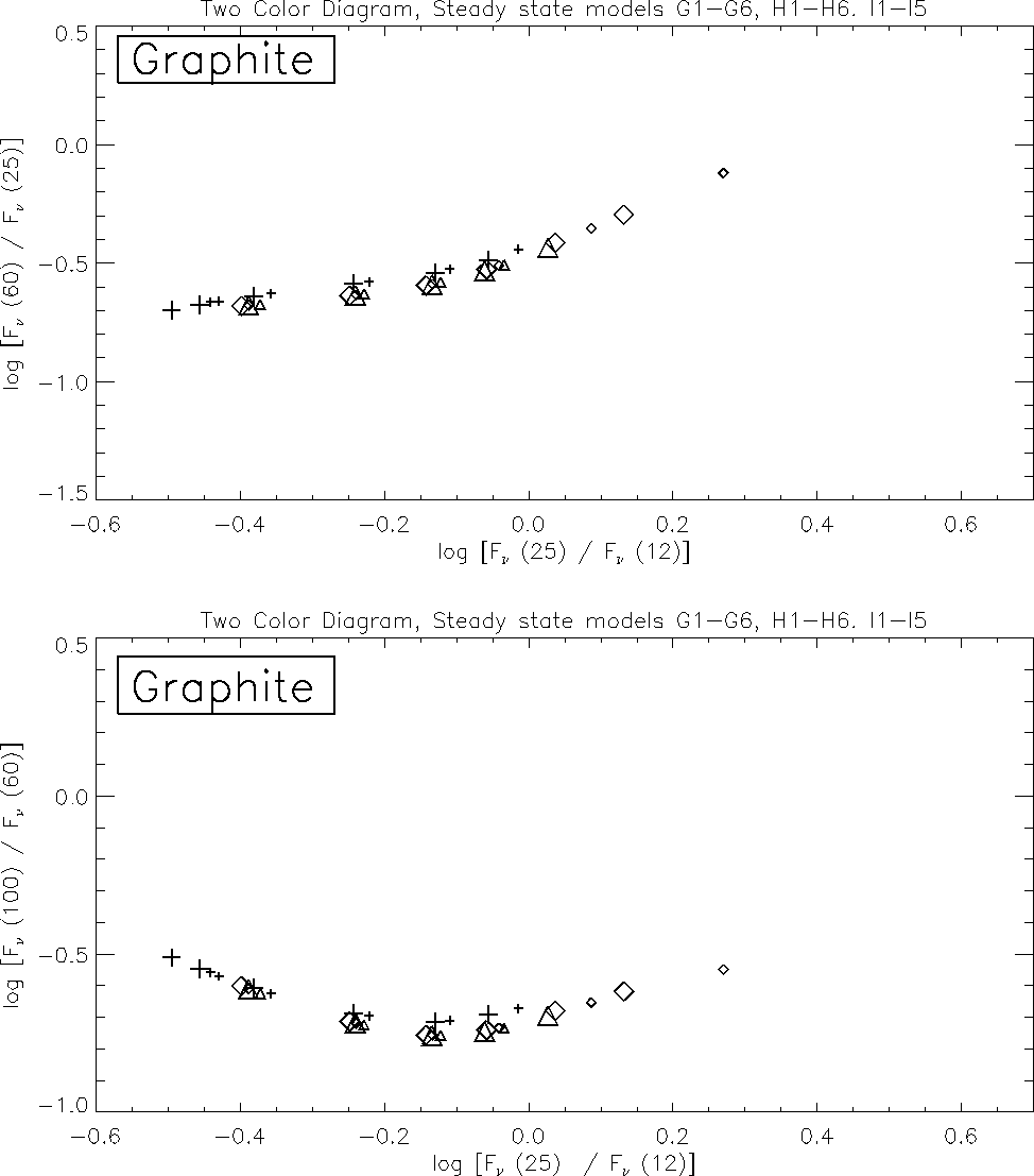
Figure 13:
Top: IRAS two-color diagram for the Carbon star models G (+), H (![]() ),
and I (
),
and I (![]() ), based on dust grains consisting of graphite.
For each large symbol, indicating the position
of a model computed with gas pressure, there is a corresponding small symbol
close to it, showing the position of the respective model computed without
gas pressure. Bottom: Same as above, but showing the flux ratio
), based on dust grains consisting of graphite.
For each large symbol, indicating the position
of a model computed with gas pressure, there is a corresponding small symbol
close to it, showing the position of the respective model computed without
gas pressure. Bottom: Same as above, but showing the flux ratio
![]() in the ordinate
in the ordinate

Figure 14:
Top: IRAS two-color diagram for the Carbon star models J (+), K (![]() ),
and L (
),
and L (![]() ), based on dust grains consisting of amorphous carbon.
For each large symbol, indicating the position
of a model computed with gas pressure, there is a corresponding small symbol
close to it, showing the position of the respective model computed without
gas pressure. Bottom: Same as above, but showing the flux ratio
), based on dust grains consisting of amorphous carbon.
For each large symbol, indicating the position
of a model computed with gas pressure, there is a corresponding small symbol
close to it, showing the position of the respective model computed without
gas pressure. Bottom: Same as above, but showing the flux ratio
![]() in the ordinate
in the ordinate

Figure 15:
Terminal gas velocity, ![]() , for different Oxygen stars obtained with our
radiation hydrodynamics code including (+) and ignoring (
, for different Oxygen stars obtained with our
radiation hydrodynamics code including (+) and ignoring (![]() ) gas
pressure in the equations of motion compared with the data given in Table 3 of
NE (
) gas
pressure in the equations of motion compared with the data given in Table 3 of
NE (![]() ) for different mass loss rates. Note that NE ignore gas
pressure. The dust is assumed to consist of grains of astronomical silicates
with
) for different mass loss rates. Note that NE ignore gas
pressure. The dust is assumed to consist of grains of astronomical silicates
with ![]() m,
m, ![]() g cm-3,
g cm-3, ![]() ,
,
![]() K. From top to bottom, the parameters are:
K. From top to bottom, the parameters are:
![]()
![]() ,
, ![]()
![]() ,
, ![]() K and
u1 = 2 km/s (C models);
K and
u1 = 2 km/s (C models);
![]()
![]() ,
, ![]()
![]() ,
, ![]() K and
u1 = 2 km/s (D models);
K and
u1 = 2 km/s (D models);
![]()
![]() ,
, ![]()
![]() ,
, ![]() K and
u1 = 4 km/s (E models);
K and
u1 = 4 km/s (E models);
![]()
![]() ,
, ![]()
![]() ,
, ![]() K and
u1 = 4 km/s (F models)
K and
u1 = 4 km/s (F models)

Figure 16:
Terminal gas velocity, ![]() , for different Carbon stars obtained with our
radiation hydrodynamics code including (+) and ignoring (
, for different Carbon stars obtained with our
radiation hydrodynamics code including (+) and ignoring (![]() ) gas
pressure in the equations of motion compared with the data given in Table 3 of
NE (
) gas
pressure in the equations of motion compared with the data given in Table 3 of
NE (![]() ) for different mass loss rates. Note that NE ignore gas
pressure. The dust is assumed to consist of grains of graphite with
) for different mass loss rates. Note that NE ignore gas
pressure. The dust is assumed to consist of grains of graphite with ![]() m,
m, ![]() g cm-3,
g cm-3, ![]() ,
, ![]() K.
From top to bottom, the parameters are:
K.
From top to bottom, the parameters are:
![]()
![]() ,
, ![]()
![]() ,
, ![]() K and
u1 = 2 km/s (G models);
K and
u1 = 2 km/s (G models);
![]()
![]() ,
, ![]()
![]() ,
, ![]() K and
u1 = 2 km/s (H models);
K and
u1 = 2 km/s (H models);
![]()
![]() ,
, ![]()
![]() ,
, ![]() K and
u1 = 2 km/s (I models)
K and
u1 = 2 km/s (I models)

Figure 17:
Terminal gas velocity, ![]() , for different Carbon stars obtained with our
radiation hydrodynamics code including (+) and ignoring (
, for different Carbon stars obtained with our
radiation hydrodynamics code including (+) and ignoring (![]() ) gas
pressure in the equations of motion. The dust is assumed to consist of grains
of amorphous carbon with
) gas
pressure in the equations of motion. The dust is assumed to consist of grains
of amorphous carbon with ![]() m,
m, ![]() g cm-3,
g cm-3,
![]() ,
, ![]() K.
For models J, triangles indicate the
K.
For models J, triangles indicate the ![]() resulting when the gas
pressure terms are computed with a molecular weight
resulting when the gas
pressure terms are computed with a molecular weight ![]() (molecular
hydrogen) instead of the standard assumption
(molecular
hydrogen) instead of the standard assumption ![]() (atomic hydrogen).
From top to bottom, the parameters are:
(atomic hydrogen).
From top to bottom, the parameters are:
![]()
![]() ,
, ![]()
![]() ,
, ![]() K and
u1 = 2 km/s (J models);
K and
u1 = 2 km/s (J models);
![]()
![]() ,
, ![]()
![]() ,
, ![]() K and
u1 = 2 km/s (K models);
K and
u1 = 2 km/s (K models);
![]()
![]() ,
, ![]()
![]() ,
, ![]() K and
u1 = 2 km/s (L models)
K and
u1 = 2 km/s (L models)

Figure 18:
Coupling factor ![]() as a function of
as a function of ![]() ,
(optical depth at
,
(optical depth at ![]() m) and
m) and ![]() (flux-averaged optical
depth; cf. Eq. 25 (click here)). Top frames: Results for our Oxygen star models
computed without gas pressure (Ci_n (+); Di_n (
(flux-averaged optical
depth; cf. Eq. 25 (click here)). Top frames: Results for our Oxygen star models
computed without gas pressure (Ci_n (+); Di_n (![]() ); Ei_n
(
); Ei_n
(![]() ); Fi_n (
); Fi_n (![]() )) and
for models Di_m (
)) and
for models Di_m (![]() ) computed with gas pressure.
Middle frames : Results for our Carbon star models with graphite dust,
computed without gas pressure (Gi_n (+); Hi_n (
) computed with gas pressure.
Middle frames : Results for our Carbon star models with graphite dust,
computed without gas pressure (Gi_n (+); Hi_n (![]() );
Ii_n (
);
Ii_n (![]() )) and for models Hi_m (
)) and for models Hi_m (![]() )
computed with gas pressure.
Bottom frames: Results for our Carbon star models with amorphous carbon dust,
computed without gas pressure (Ji_n (+); Ki_n (
)
computed with gas pressure.
Bottom frames: Results for our Carbon star models with amorphous carbon dust,
computed without gas pressure (Ji_n (+); Ki_n (![]() );
Li_n (
);
Li_n (![]() )) and for models Ki_m (
)) and for models Ki_m (![]() )
computed with gas pressure. The dotted diagonal in the right-hand frames
indicates the relation
)
computed with gas pressure. The dotted diagonal in the right-hand frames
indicates the relation ![]() , the maximum slope
attainable by high luminosity models without gas pressure
, the maximum slope
attainable by high luminosity models without gas pressure