3. The PHEMU91 campaign

Table 1 (click here) gives the list of the names, longitudes and latitudes of the sites from which the mutual events were observed and Table 2 (click here) gives the list of the receptors used for the recording of the observations. Several kinds of receptors were used for the observations:

1. photometric receptors,
2. two-dimensional receptors,
3. visual observations.

They were used with reflector and refractor telescopes, many of which had small apertures since the Galilean satellites are about magnitude 5. A filter (specified in the data) was used in most cases.

3.1. Photometric receptors

These receptors are currently used for absolute photometry. In the case of the mutual events, only relative photometry is necessary. Anyway, since the elevation of Jupiter above the horizon may be very small, absolute photometry is not possible: the air mass is often too large. The description of some photometers that we used is as follows:

1. At Paris Observatory (France), behind a 38 cm-refractor, an uncooled RCA 4840 photomultiplier (multialcali photocathode) the sensitivity of which is from 350 to 750 micrometers. This equipment is described by Briot (1987) and will be denoted "PM9" in the data tables.
2. At CERGA (Observatory at Calern near Grasse, France) behind a 150 cm reflector, the photometer TELOC at 450 micrometers, described by Froeschlé et al. (1988) and denoted "POB" for channel B, "POV" for channel V, "POR" for channel R in the data tables.
3. At Teramo Observatory (Italy), behind either a 40 cm refractor or a 50 cm reflector, an EMI 6256A or a 6256SA described by Burchi & Di Paolantonio (1987) and denoted "PM4" in the data tables.
4. At Catania Observatory (Italy), behind a 91 cm-reflector, a cooled photon counting single-head photometer equipped with an EMI 9789QA photomultiplier described by Blanco et al. (1991) and denoted "PM2" in the data tables.
5. At GEA (Grup d'Estuds Astronomics) several telescopes were used the apertures of which varied from 20 to 41 cm. Two types of photometers were used: either a photodiode photometer OPTEC-SSP3 denoted "PM5" in the data tables, either a photomultiplier HPO (1P21) or an OPTEC SSP-5 (Hamamatsu R1414) denoted "PM17" in the data tables. The telescopes were used either in the Pyrenean mountains or in the vicinity of Barcelona (Spain). The description of the equipment is given by Gomez-Forrellad (1987).
6. At the European Southern Observatory (La Silla, Chile), behind either a 50 cm or a 1 m reflector, two photometers were used: either a EMI 6256(S-13) or a Quantacon RCA-31036 (Ga-As) denoted "PM4" and "PM3" in the data tables. The description is given by Gouiffes et al. (1987).
7. At Brasopolis Observatory (Brazil), behind a 60 cm reflector, a cooled Hamamatsu 943-02 denoted "PM15" in the data tables.
8. At Mauna Kea (Hawaii, U.S.A.), a dry ice cooled RCA C31034A photomultiplier behind a 61 cm-reflector denoted PM16. The filter was a H2O+ from the IHW filter set.
9. At Jungfrau Observatory (Switzerland), behind a 76cm telescope, a cooled photomultiplier photometer (with a S11 cathode) denoted "S11" in the data tables.
10. Some amateur astronomers used also photometers. At Zoetermeer (Netherlands), an OPTEC photodiode photometer was used (denoted "PM14" in the data tables), as well as at Essen (Germany) and Holtsville (U.S.A.) where photodiode photometers denoted "PM5" were used.

The data tables, give also the nature of the filter used as well as the observational conditions for each event.

 

Longitude Latitud e elevation

Main observatories h m s meters

Barcelona (GEA-Spain) 0 8 39.7 E 41 23 54 N 19

Belogradchik (Bulgaria) 1 30 42.0 E 43 37 35 N 630

Beograd (Yugoslavia) 1 22 3.0 E 44 48 12 N 260

Berlin (Germany) 0 53 40.0 E 52 32 0 N 82

Bordeaux (France) 0 2 6.6 W 44 50 7 N 73

Bowie, Maryland (U.S.A.) 5 7 31.3 W 38 58 55 N 200

Brasopolis (Brazil) 3 2 16.0 W 22 31 6 S 1870

Bucarest (Romania) 1 44 23.1 E 44 24 50 N 80

Calern (CERGA-France) 0 27 41.2 E 43 45 17 N 1282

Catania (Italy) 0 59 55.0 E 37 41 30 N 1725

Cluj-Napoca (Romania) 1 34 23.0 E 46 42 48 N 750

Devon Obs. (Canada) 7 35 2.0 W 53 23 26 N 500

Jungfrau (Swizerland) 0 31 56.4 E 46 32 53 N 3578

Kakuda (Japan) 9 24 0.0 E 38 0 0 N 17

Kavalur VBO (India) 5 15 19.6 E 12 34 32 N 725

La Silla (ESO-Chile) 4 42 55.1 W 29 15 25 S 2347

Mauna Kea (Hawaii, U.S.A.) 10 21 7.2 W 19 50 0 N 4215

Meudon (France 0 8 55.5 E 48 48 18 N 162

Mollet (GEA-Spain) 0 8 50.0 E 41 32 22 N 70

Nice (France) 0 29 19.1 E 43 43 17 N 376

OHP (France) 0 22 52.0 E 43 55 46 N 665

Paris (France) 0 9 20.9 E 48 50 11 N 67

Pic-du-Midi (France) 0 0 34.2 E 42 56 12 N 2861

Reggio Calabria (Italy) 1 2 36.4 E 38 6 25 N -

Reux (Belgium) 0 20 21.8 E 50 14 43 N 317

Rio de Janeiro (Brazil) 2 52 53.6 W 22 53 44 S 33

Siding Spring (Australia) 9 56 16.0 E 31 17 0 S 1145

Tenerife (Canarian Islands,Spain) 1 6 20.0 W 28 15 0 N 2400

Teramo (Italy) 0 54 56.0 E 42 39 30 N 388

Timisoara (Romania) 1 24 55.0 E 45 44 15 N 88

Tokyo (Japan) 9 18 0.0 E 35 40 0 N 58

Zoetermeer (The Netherlands) 0 17 55.1 E 52 04 11.6 N 5

 

3.2. Two-dimensional receptors

Another interesting type of receptors is the two-dimensional ones. In fact, these receptors record images in place of light-flux. Depending on the receptor, it is possible to calculate the light-flux of the satellites during the event. However, several problems have to be solved. The most important is the speed of acquisition of the images. The time constant depends on the duration of the event but should be, most of time, less than one second of time. Some receptors are not able to acquire images so fast. The receptors that we used are as follows:

1. cooled CCD (c.) driven by a computer; images are directly recorded as numerical arrays of pixels and the calculation of the light-flux, the reduction using reference objects and the sky background is easy. However, the time constant is often large and we will get a small number of points for the light-curves. For long events, it will be very favorable since the noise will decrease. We note that faster computers and better softwares will permit much higher frequency acquisition for the next campaigns of observations. The receptors used are denoted "CCD1" for the one built by Bordeaux Observatory and described by Le Campion et al. (1992), "CCD2" for the one built by Pic-du-Midi Observatory and described in Colas (1995), "CCD3" for the one used by Mallama and described in Mallama (1992) and "IR-A" for the infrared array used at CRL, Tokyo and described in Souchay et al. (1992).
2. video mode uncooled CCD (unc.); images are recorded on a VCR as an analogic signal. Because of the large speed of acquisition (25 images per second, integrating time 0.02 second), the sensitivity is smaller than with a cooled CCD driven by a computer. So, a light intensifier may be used in front of the CCD target. The reduction is made by digitizing the images and by analyzing the numerical arrays of pixels. Such a digitizing technique is described by Arlot et al. (1989). These receptors are denoted "CCDVn" in the tables. Note than an intensified tube camera (SIT Vidicon) denoted "N" was also used in video mode.
3. the photographic technique may also be used as a two-dimension receptor but the sensitivity is very low and the time constant very large. When used, such a technique has been denoted "PH" in the tables.

  
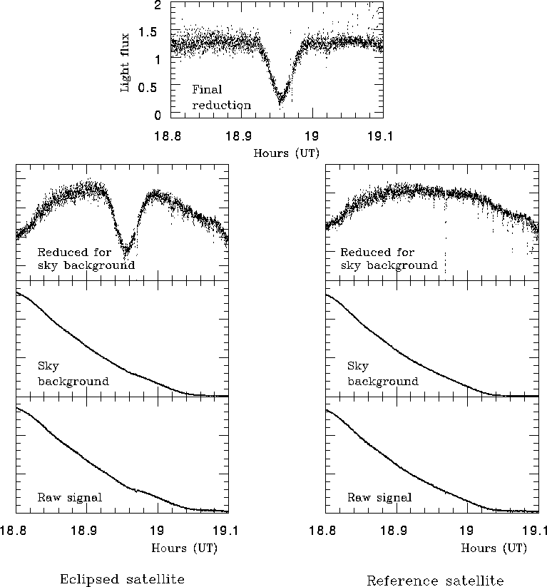
Figure 2: Observation of the eclipse of J2 by J1 at Meudon Observatory on April 22, 1991

As an example, Fig. 2 (click here) shows how the reduction is performed for an event recorded using a two-dimensional receptor. This event has been observed at Meudon Observatory in very difficult local conditions with a video mode CCD camera. It was twilight and some light clouds were passing in front of Jupiter during the event. The raw signal shows evidently the decreasing twilight. After substracting the sky background, all the recorded objects show the variation of the transparency of the sky due to the clouds. Using a reference constant object, the light curve resulting from the reduction has the shape that we were looking for.

3.3. Visual observations

We give also visual lightcurves (denoted "V" in the data tables). They were obtained in most case using the Argelander method (Dumont & Figer 1973). The magnitude scale is arbitrary and only the date of the minimum of the light curve is available from these data. Most of time, the time accuracy is better than one second of time. Very little information will be provided by the means of these light curves. However, in some cases, they may be helpful for analysis and comparison with the other ones. Note that most of the observers belong to the GEOS association (Groupe Etudes et Observations Stellaires).