4. Calibration algorithm for theoretical library spectra

We now establish a correction procedure for the library spectra which preserves their detailed features but modifies their continua in such a way that the synthetic colors from the corrected library spectra conform to the empirical color-temperature relations. Since the empirical color-temperature relations do not provide direct access to the stellar continua, pseudo-continua are instead being calculated for each temperature from both the empirical (Table 2 (click here)) and the theoretical (model-generated) colors. The ratio between the two pseudo-continua then provides the desired correction function for the given .

  
Figure 8: Black-body fit of temperature to a synthetic spectrum for , illustrating the least-squares solution of Eqs. (3). The crosses represent the integrated (heterochromatic) fluxes of the synthetic spectrum measured in the different (broad) bandpasses

4.1. Pseudo-continuum definition

For a given stellar flux spectrum of effective temperature , we define the pseudo-continua as black bodies of color temperature varying with wavelength:

where is a scale factor and is the black body function, both of which need to be determined by least-squares fits of to the broad-band fluxes of the given flux spectrum. Thus,

where S_i is the normalized transmission function of the passband i and f_i is the broad-band flux measured through this passband. Because colors are relative measurements, we normalize by arbitrarily setting the absolute flux in the I-band to be equal to 100: f_I=100. The black-body fit in Eq. (3) is then obtained iteratively by a conjugate gradients method.

Figure 8 (click here) illustrates a typical result. Note that, because effects of blanketing are ignored by this fitting procedure, the mean temperature, , associated with the best-fitting black-body curve, is systematically lower than the effective temperature of the actual flux spectrum.

having thus been determined, the color temperatures, , can be derived in a straightforward manner at the mean wavelengths of the passbands i via the equations:

Interpolation between the by a spline function finally provides the continuous (and smooth) color temperatures (Fig. 9 (click here)) required to calculate the pseudo-continua defined by Eq. (2).

4.2. Correction procedure

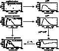
The correction procedure is defined by the following sequence, and is illustrated (steps 1 to 4) in Fig. 10 (click here).

1. At effective temperature , the empirical pseudo-continuum is computed from the colors of the empirical temperature-color relations given in Table 2 (click here).
2. At the same effective temperature , the synthetic pseudo-continuum is computed from the synthetic colors obtained for the original theoretical solar-abundance spectra given in the K- and/or -libraries:
   
   where is defined in the same way as in Sect. 3 by a evolutionary track calculated by Schaller et al. (1992).
3. The correction function is calculated as the ratio of the empirical pseudo-continuum and the synthetic pseudo-continuum at the effective temperature :
   
   
4. Corrected spectra, , are then calculated from the original library spectra, :
   
   Note that the correction defined in this way becomes an additive constant on a logarithmic, or magnitude scale. Therefore, at each effective temperature the original monochromatic magnitude differences between model library spectra having different metallicities [M/H] and/or different surface gravities are conserved after correction. As we shall see below, this will be true to good approximation even for the heterochromatic broad-band magnitudes and colors because, as shown in Fig. 11 (click here), the wavelength-dependent correction functions do not, in general, exhibit dramatically changing amplitudes within the passbands.

   Figure 11 (click here) shows how the resulting correction functions change with decreasing effective temperature. Finally, Figs. 12 (click here) and 13 (click here) display the corresponding effective temperature sequence of original and corrected spectra at different metallicities for the full (Fig. 12 (click here)) and the visible (Fig. 13 (click here)) wavelength ranges, respectively.

     
   Figure 9: Color temperatures for synthetic spectra covering a range of effective temperatures, as labelled. Top pair: K-library dwarf models; middle pair: K-library giant models; bottom pair: -library giant models. Note that systematically , as tracked down by the black-body fit temperatures,
   

5. Finally, the normalization of fluxes in the I-band, f_i=100, adopted initially for calculating the pseudo-continua must be cancelled now in order to restore the effective temperature scale. Thus, each corrected spectrum of the library, is scaled by a constant factor, , to give the final corrected spectrum :
   
   where
   
   assures that the emergent integral flux of the final corrected spectrum conforms to the definition of the effective temperature (Eq. (1)).

  
Figure 10: Correction procedure. All fluxes are normalized to f_I=100

The final corrected spectra are thus in a format which allows immediate applications in population evolutionary synthesis. For a stellar model of given mass, metallicity, and age, the radius R is determined by calculations of its evolutionary track in the theoretical HR diagram, and the total emergent flux at each wavelength can hence be obtained from the present library spectra via